Induction heating — a frequency sweep that becomes a thermal transient

← Back to the examples

What you need to run it: the Python API (Automation), plus Core Pro for the time-harmonic simulation type and Crank-Nicolson, and the Thermal module for the last stage. The script prints which module unlocks which stage before it builds anything, so an unlicensed reader learns what the example would have shown rather than watching it fail halfway.

What this one is for

This is the set's time-harmonic example and its thermal example, and the two are the same run: the induced power the electromagnetic sweep measures is what heats the billet in the second half. If you want to see why the frequency domain exists — and what an honest handoff from an electromagnetic result to a thermal one looks like — this is the page.

The device is a stainless-steel billet inside a six-turn water-cooled copper induction coil, axisymmetric, with the solver integrating over 2π. So every power below is the power of the whole billet, not a per-metre figure.

At a glance

Quantity	Value	Unit
Billet	Ø40 × 120, AISI 304 (σ = 1.4e6 S/m, μr = 1)	mm
Coil	6 turns of 10 × 10 square tube, ID 56, 25 pitch	mm
Drive	250 peak, at 1 / 5 / 10 / 30 kHz	A
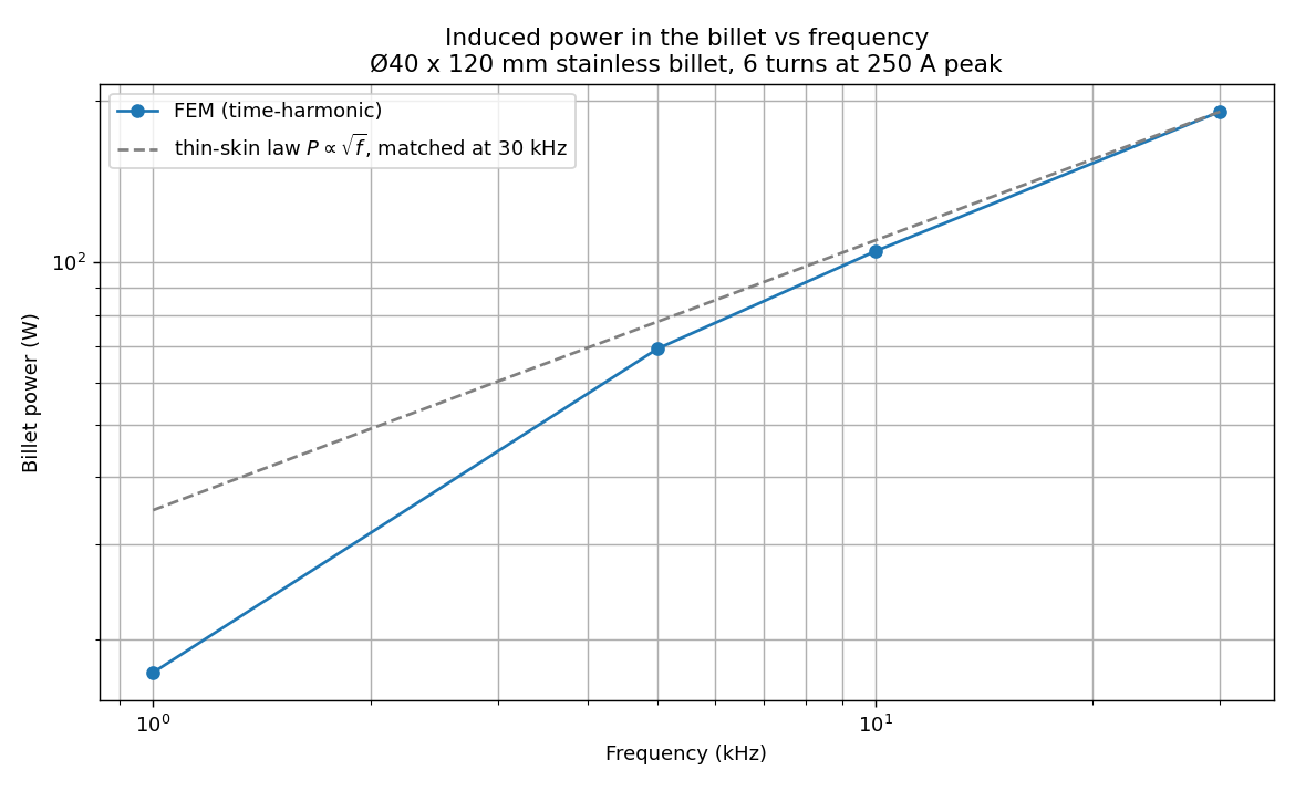
Induced power at 1 / 5 / 10 / 30 kHz	17.39 / 69.32 / 105.00 / 190.50	W
Time-harmonic vs settled transient at 10 kHz	105.00 vs 106.31 W, 1.25 (tol 5)	%
Skin depth measured vs analytic, 10 / 30 kHz	+12.0 / +8.4 (tol 15)	%
Steady surface / centre temperature	318.5 / 327.0	°C
Thermal energy balance	0.02	%
Thermal time constant	1693 (28.2 min)	s
Mesh	13746 EM nodes, 1027 thermal nodes	—
Wall time	20 (of which ~8 is JVM startup)	s

Stage 1 — time-harmonic used as the tool it is

One mesh, four solves. The geometry, the mesh and the excitation are fixed, so an operating point costs one complex solve of (K + jωM)Â = F̂ instead of forty transient steps that then have to be checked for settling. Measured on this model: the whole four-point sweep is 11 s; the settled transient of one of those points adds 130 s.

The thin-skin law is P ∝ √f, because the induced power per unit surface is Hrms²/(σδ) and δ ~ 1/√f. The reference line is anchored at 30 kHz deliberately, because the visible result is the 1 kHz point falling to half of it — where δ = 13.4 mm is no longer small against the 20 mm radius and the thin-skin picture has stopped applying.

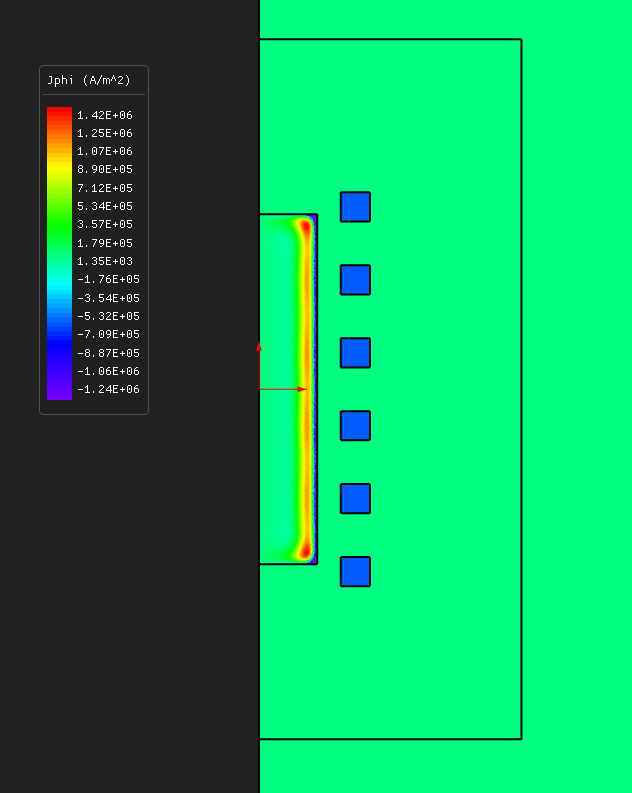
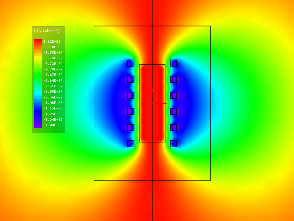
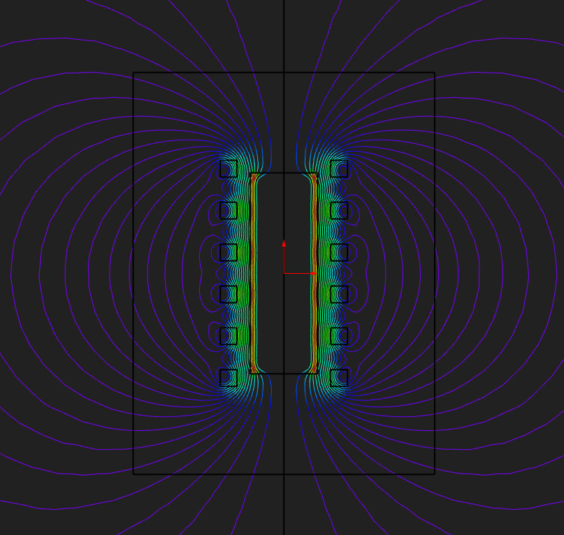
The coil turns as sources, the billet's skin as the reaction, and the flux lines being pushed out of the billet.

The skin depth, and why only two points are checked

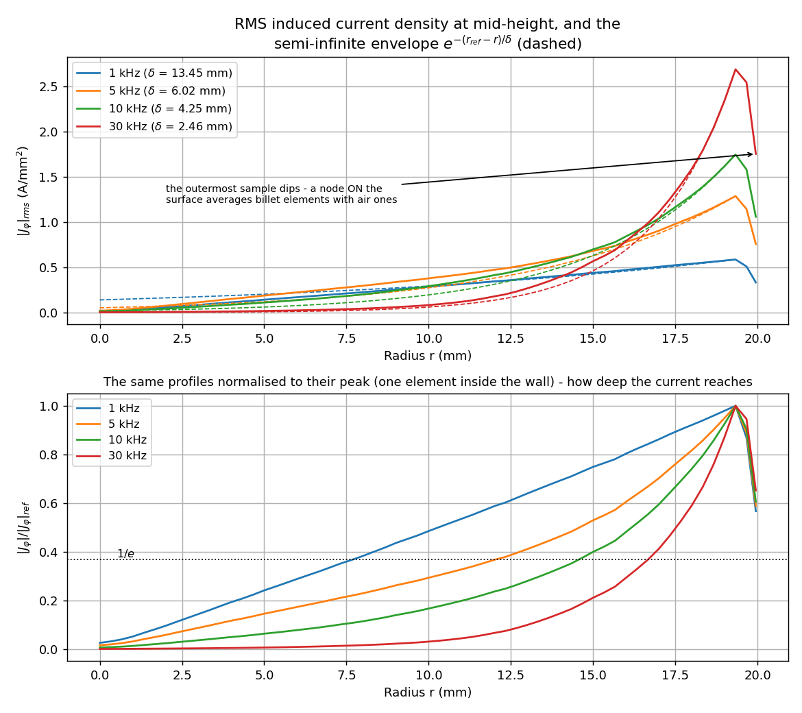
f	Analytic δ	Measured
1 kHz	13.45 mm	11.64 mm	−13.4 %	not checked
5 kHz	6.02 mm	7.31 mm	+21.5 %	not checked
10 kHz	4.25 mm	4.77 mm	+12.0 %	tolerance 15 %
30 kHz	2.46 mm	2.66 mm	+8.4 %	tolerance 15 %

Two things about that table are the point, and neither is tuned away.

The measured depth runs long by construction, and more so the thicker the skin. δ is the semi-infinite slab answer. In a cylinder the exact profile falls off a little more slowly than the slab formula says, so the 1/e depth comes out long — a few percent when the skin is an eighth of the radius, about twenty percent when it is a third. That is why only the two thin-skin points are checked: at 1 and 5 kHz the semi-infinite formula is not a slightly-wrong model of this billet, it is the wrong model, and the run says so instead of widening a tolerance until it passes.

Part of the remaining bias is mesh, and it is measured. Quartering the billet mesh (42 229 nodes instead of 13 746) moves 10 kHz from +12.0 % to +9.6 % and 30 kHz from +8.4 % to +3.7 %. What is left is the geometry.

One subtlety in that measurement. The reference is the profile's maximum, not its outermost sample — visible in the figure as a dip in the last point. A point probe reads the nodal field, which is averaged over every element sharing the node, so a node sitting on the billet surface averages billet elements carrying the full induced current with air elements carrying none, and reads about 30 % low. The maximum sits one element inside the wall, past that averaged layer. The same trap catches any probe placed on a material interface.

The transient that makes the cheap number believable

A time-harmonic answer is a claim about the steady state, and the honest way to test it is to march to that steady state. Two settings carry the run and neither is decoration. Crank-Nicolson, because Backward Euler damps an AC eddy-current problem and the damping is a loss error — the very number being compared. And twenty periods, because the billet's bulk diffusion time is seven periods at 10 kHz and it is the initial transient that has to decay through it; the loss is averaged over the last two periods only.

cross-check at 10 kHz: time-harmonic 105.00 W vs settled transient 106.31 W (1.25%, tol 5%)
                       - 801 transient steps against one complex solve

The electromagnetic-to-thermal handoff

Nabla's thermal module is uncoupled. It solves conduction on a mesh with the heat sources you give it; it does not read the electromagnetic solution. So the handoff here is manual and explicit — and presenting it as a two-way coupled solve would misrepresent the product. Written out, it is three lines:

q = power_W / billet_volume_m3()   # 105.00 W / 150.8 cm^3 = 6.96e5 W/m^3
model.setThermalEnabled(True)
model.setThermalRegionProperty("Billet", "q", q)

The thermal domain is the billet alone, and the air around it is not part of it. That is not a shortcut either: air is not a conduction path worth solving, and a convection boundary condition is a statement about a surface that has to be a boundary of the mesh. So stage 3 builds its own small model — the billet rectangle, 1027 nodes — with convection on the three real faces and nothing on the axis, where a natural zero-flux edge is the symmetry condition.

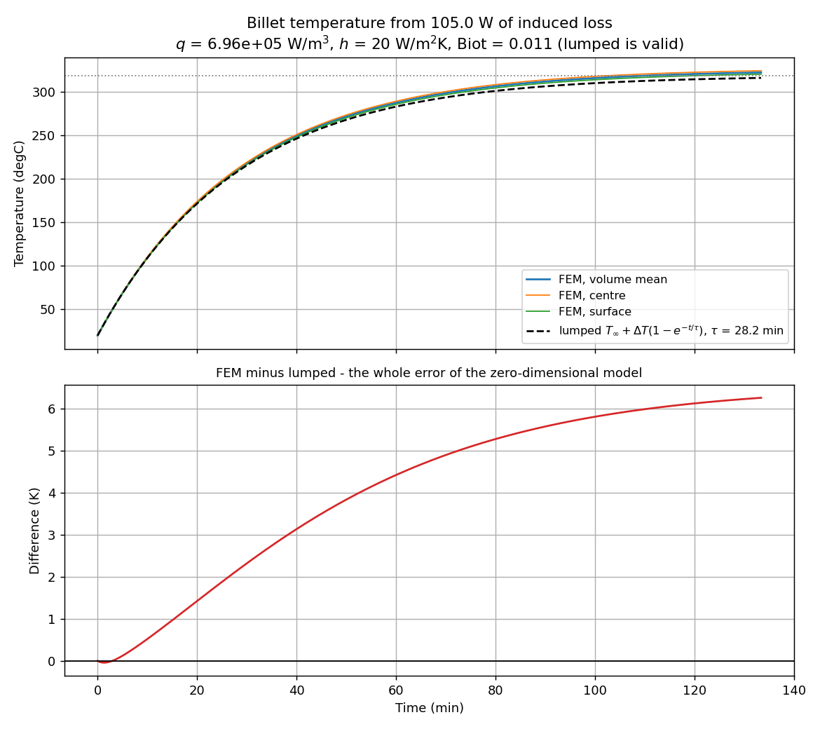
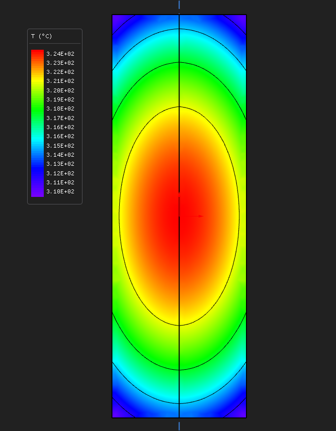
steady state: surface 318.5 degC, centre 327.0 degC;
              h*A*(Ts-Tinf) = 105.02 W vs q*V = 105.00 W  (0.02%)
time constant tau = rho*cp*V/(h*A) = 1693 s = 28.2 min; steady rise 298 K -> 318 degC

Three checks close to better than 2.2 %. The steady-state energy balance is 0.02 % — close to an identity the FEM enforces, which is the point: what it actually tests is that the axisymmetric 2π revolve of a volume and of a surface are consistent with each other and with the q that went in. The early slope dT/dt = q/(ρcp), when nothing has left yet, is 1.28 % off. And the whole curve against lumped capacitance is within 2.10 % of the 298 K steady rise — the Biot number is 0.011, so the billet is thermally thin and the two must agree; the 6 K the FEM sits above the lumped model at equilibrium is the internal conduction rise the zero-dimensional model has no room for.

Caveats, stated rather than tuned away

• The default mesh under-reads the highest frequency by about 3.6 %. It puts 3.9 elements inside the 2.46 mm skin depth at 30 kHz; quartering it moves 30 kHz by +3.6 %, 10 kHz by +1.3 % and 1 kHz by +0.2 %. Under-resolve a skin and the J²/σ integral reads low. The default is the accuracy-against- wall-time trade this example ships.
• The Dirichlet box has to sit far out. A solenoid's external field is dipole-like, so squeezing the box squeezes the flux and the truncation error lands straight on the induced power. Measured: a 110 mm domain reads 6 % low, 180 mm 1.6 % low, and the shipped 320 mm is within 0.3 % of 520 mm. The far air is meshed coarsely, so the honest domain costs only about 800 extra nodes.
• The heat source is uniform over the billet, computed as P/V, while the loss itself lives in the skin. For this billet that hardly matters — the surface-to-centre rise for uniform generation is 4.6 K against a 298 K bulk rise. On a poorer conductor, a thinner skin or a much larger rise it would, and the way to do it is to split the billet into a shell and a core in both models and read the Joule loss per region.
• h = 20 W/m²K is still air, and it is what makes the equilibrium land at a plausible 318 °C for this power. It is a boundary condition, not a computed film coefficient; Nabla does not solve the fluid.

The billet is austenitic on purpose. 304 is paramagnetic to better than a percent, so the skin depth is a single number the run can be checked against. A magnetic carbon steel has no single δ: μ_r falls with H through the skin and vanishes above the Curie point, which is a real and important effect in industrial billet heating and the wrong thing for an example whose job is to make the formulation checkable.

Running it

python induction_heating_axi.py                 # sweep + thermal, ~20 s
python induction_heating_axi.py --cross-check   # ... plus the settled transient (+130 s)
python induction_heating_axi.py --stage thermal # re-run the thermal stage from sweep.json
python induction_heating_axi.py --coarse        # every mesh area x4, 13 s

Try this next

• Raise the frequency, and raise the billet mesh resolution with it — the rule of thumb the default is set by is about four elements per skin depth at the top frequency.
• Change the billet material. A better conductor is a thinner skin and, for the same H, less power. Aluminium has a 0.49 mm skin depth at 30 kHz, which this mesh cannot resolve — and that is the lesson.
• Turn the convection coefficient up. The equilibrium is P/(hA) above ambient and the time constant is ρcpV/(hA), so raising h lowers both and the thermal run has to get shorter with it.

About these numbers

This is a demonstration billet and coil, not an industrial heater. Every figure on this page came out of the run described here at the settings the script ships with. For accuracy against a stated reference and tolerance, the validation dossier is where that question belongs.