Examples
Machine models that ship with Nabla, each rebuilt from nothing by the script beside it.
The machine example library
These are complete, working machine models, not fragments. Each one ships with
Nabla under examples/ as a model file, a Python script and a
write-up. Open the model and press Solve, or run the script and watch it build
the machine from an empty document — geometry, winding, materials, mesh,
solve, figures and a PDF report.
Pick one by what you are trying to do. E01 is the fastest way to see a PMSM solve end to end. E02 has the dq performance workflow. E04 and E06 draw their own rotors. E07 and E08 are induction machines, where the rotor current is part of the solve. Every page tells you what to look at, which numbers are solid, which are near the resolution limit, and what to change if you want to explore.
The designs are plausible but invented, so treat them as worked examples rather than as evidence of accuracy. For accuracy, the validation dossier states a reference and a tolerance for every case before it runs, and publishes the failures alongside the passes.
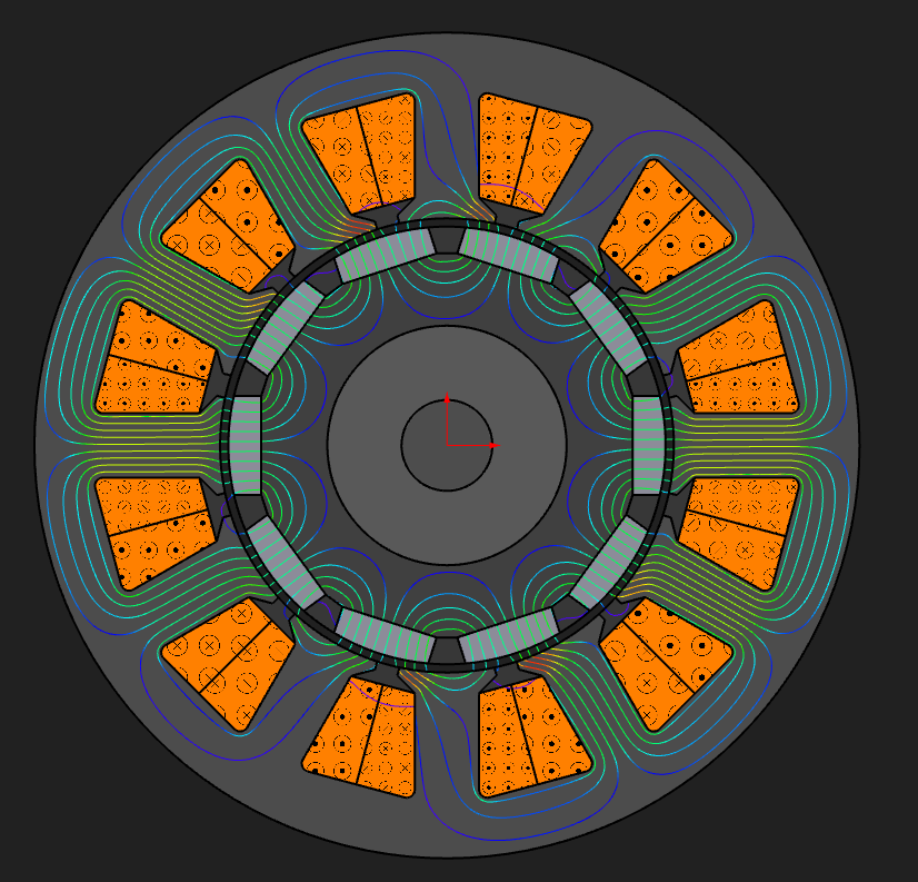
E01 — 12-slot / 10-pole surface-PM synchronous machine
PMSM · Concentrated, double layerStart here. A small surface-magnet servo motor that solves in under a minute and shows the three results a PMSM is judged on: cogging torque, back-EMF and torque under load. Repeats itself at second order for comparison.
View example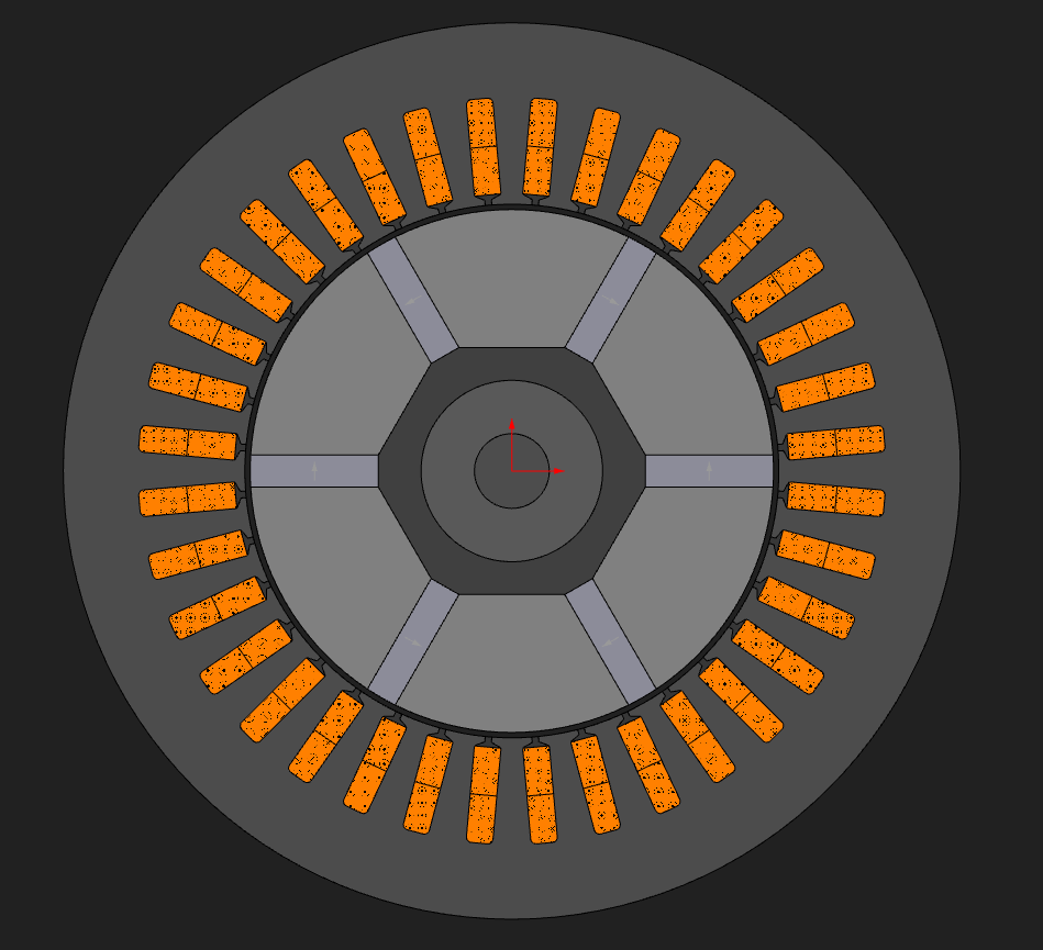
E02 — 36-slot / 6-pole spoke-type PM synchronous machine
PMSM · Distributed, double layer, 5/6 pitchA 5 kW spoke-rotor machine and the full dq workflow that goes with it - saliency, an MTPA current angle, efficiency and loss maps, fitted iron loss and a mass breakdown.
View example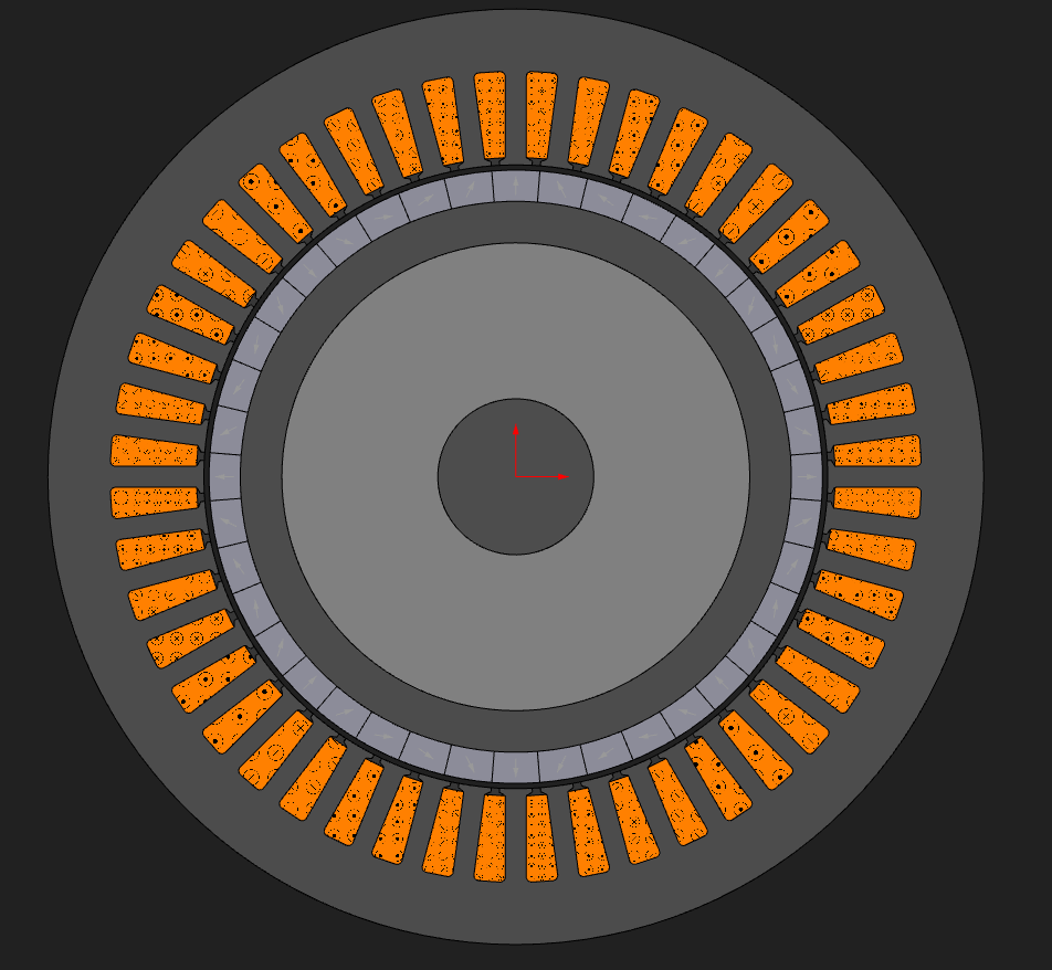
E03 — 48-slot / 8-pole segmented-Halbach PM synchronous machine
PMSM · Distributed, single layer, 4 parallel branchesThree construction choices you can see in the field: a segmented Halbach magnet array, stator skew solved as five axial slices, and a phase wound as four parallel branches. Includes a five-phase variant.
View example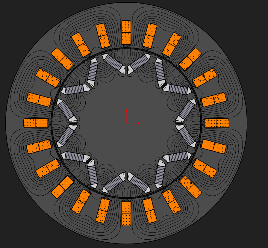
E04 — 24-slot / 8-pole V-shape interior-PM synchronous machine
PMSM · Distributed, double layer, full pitch (q = 1)A 15 kW traction-style motor with the magnets buried in a V, where a third of the torque is reluctance torque. Draws its own rotor as a DXF, and shows demagnetisation risk and magnet eddy currents.
View example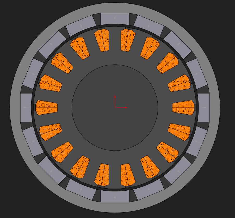
E05 — 18-slot / 16-pole surface-PM outrunner, 45 mm across, 20 000 rpm
PMSM - Outrunner · Concentrated, double layer, q = 0.375A 45 mm drone-class outrunner at 20 000 rpm, where iron loss is the larger half of the loss budget rather than a footnote. Inverted geometry, and iron loss fitted to a table that reaches 3 kHz.
View example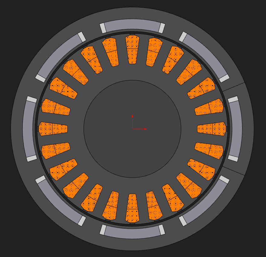
E06 — 24-slot / 8-pole interior-PM outrunner on a drawn rotor, 120 mm across
PMSM - Outrunner · Distributed, double layer, full pitch (q = 1)A 2.5 kW direct-drive outer-rotor motor with buried magnets, drawn into the annular rotor band. The two harder routes - outrunner and custom rotor - in one model.
View example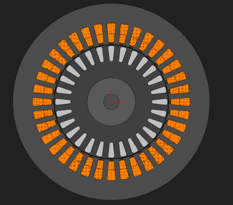
E07 — 36-slot / 28-bar 4-pole squirrel-cage induction machine
IM · Distributed, double layerThe first induction machine: a 28-bar squirrel cage whose rotor current is solved rather than imposed, with the T-equivalent circuit extracted and the torque, current, power-factor and efficiency curves swept against slip.
View example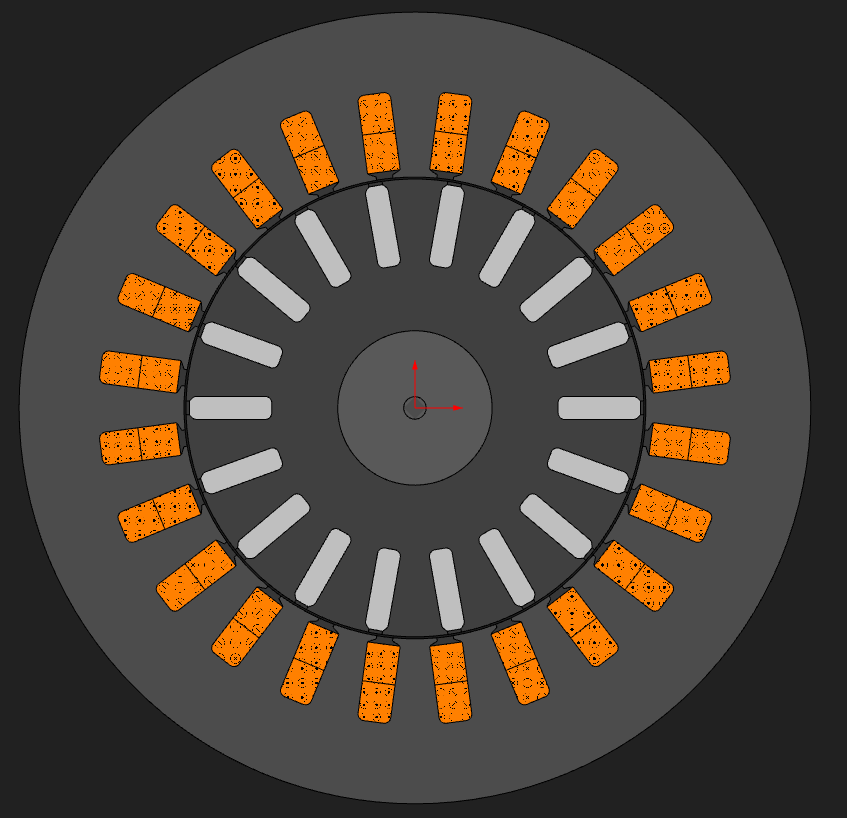
E08 — 24-slot / 18-bar 4-pole induction machine with skewed rotor bars
IM · Distributed, double layerSkewed rotor bars solved as three coupled axial slices, on a deep bar where the skin effect matters. The slowest model here, and the one that shows what skew costs and what it buys.
View exampleBeyond machines
Nabla is not only a machine tool, and none of these is a machine. Each one is a plain geometry model — lines, circles, regions, coils, boundary conditions — built from an empty document by a single Python script, with no machine module involved anywhere. Between them they cover the whole solver: static, transient, time-harmonic and thermal; planar and axisymmetric; permanent magnets, eddy currents, external circuits, motion and the far-field boundary. They are also the shortest way to see the shape of an API script before committing to a rotor.
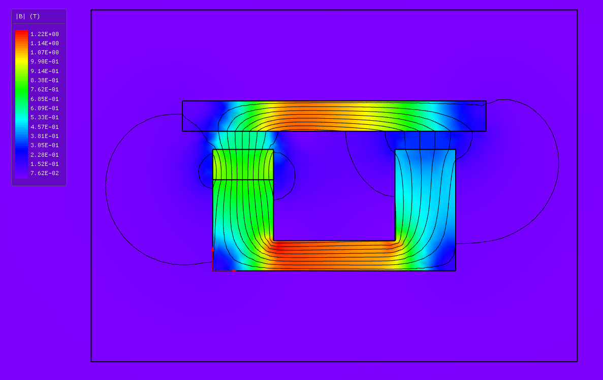
Magnet latch — pull-off force and the far-field boundary
Non-machine · Planar static · No coil, no currentThe simplest device here and the only one whose sole source is a magnet's own remanence. A gap sweep against the classical permeance model - which it misses by 34 %, for two reasons it names - and the far-field balloon boundary condition measured against a 20× Dirichlet box.
View example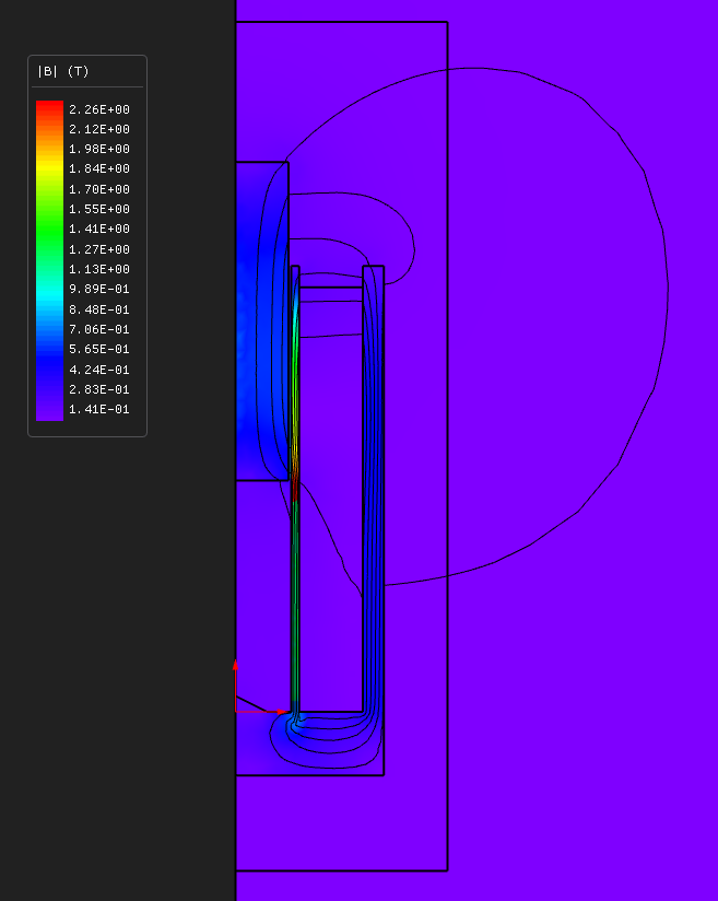
Solenoid actuator — force and inductance over the stroke
Non-machine · Axisymmetric staticThe axisymmetric primer: model x is the radius, the solver integrates over 2π, and there is no axial length to set. The eggshell force is cross-checked against the virtual-work derivative of the device's own inductance curve - and the example is precise about where that check works and why.
View example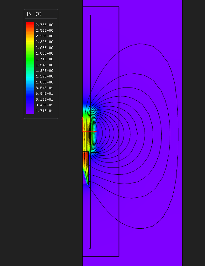
Gauss gun — a coilgun from force map to muzzle velocity
Non-machine · Axisymmetric · Static + transient + circuit + BHThe largest of these: one script using the static solver, the transient solver, an external circuit and a nonlinear BH curve on the same device, then integrating the mechanics in Python and measuring the error of having done so. The turn-off timing sweep is the figure that pays for it.
View example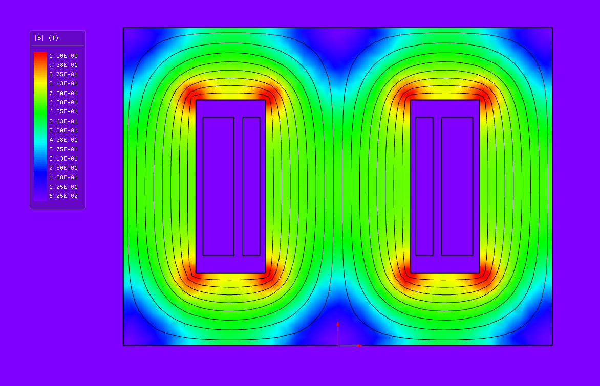
Single-phase transformer — a hand-built coil on a hand-built netlist
Non-machine · Planar transient, circuit-coupledThe circuit-coupling reference: what you copy to drive your own windings from your own netlist. Two galvanically isolated loops tied only by the core flux - and a measured demonstration that turning saturation off does not make a BH core linear at its operating point.
View example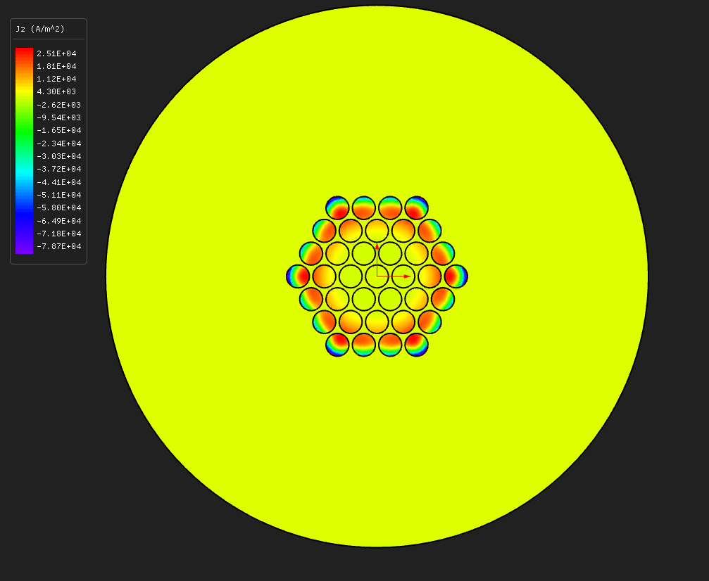
Cable AC loss — skin and proximity effect in a stranded cable
Non-machine · Transient and time-harmonicThirty-seven copper strands driven identically, and at 10 kHz the outermost ring does nearly all the work while the middle of the bundle goes dark. Parametrized strand count, and the same model solved twice - three periods of transient and one frequency-domain solve - to compare the two.
View example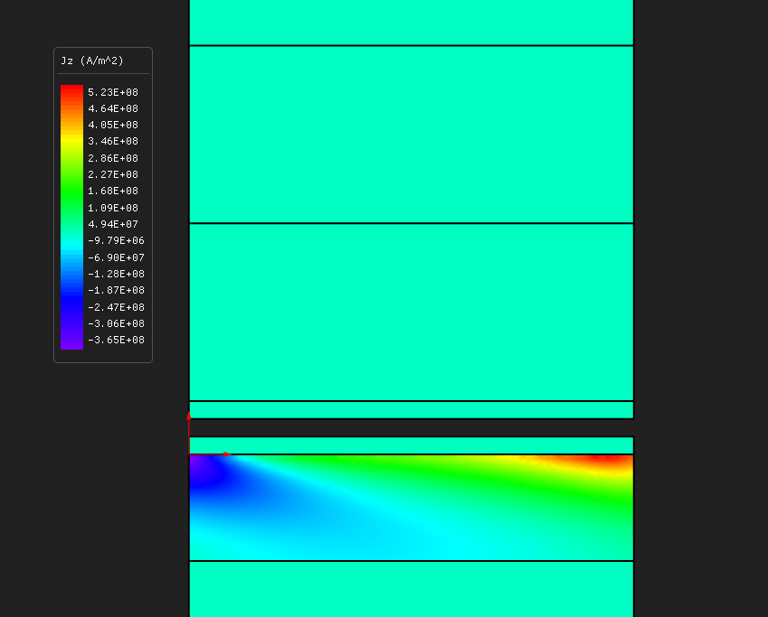
Eddy-current brake — drag against speed, through a sliding band
Non-machine · Planar transient with linear motionThe motion demo, and the only one whose eddy currents come from movement rather than an AC source: no impressed current anywhere, just magnets and a sliding rail. Drag peaks and then falls as the currents start shielding the rail - and the three sliding-band rules are written out where they apply.
View example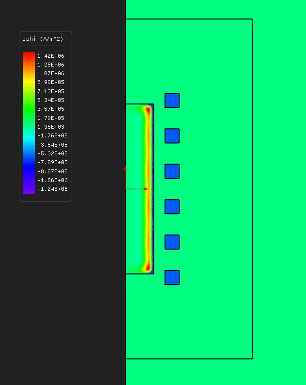
Induction heating — a frequency sweep that becomes a thermal transient
Non-machine · Axisymmetric time-harmonic + thermalWhy the frequency domain exists: four operating points as four complex solves, where the settled transient of one of them costs six times the whole sweep. Then the measured induced power is handed to the thermal module - explicitly, because Nabla's thermal solve is uncoupled - and heats the billet to equilibrium.
View example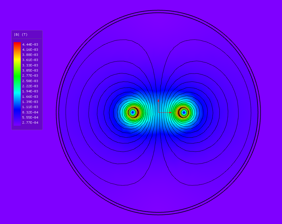
Magnetic shield — mu-metal against aluminium, 1 Hz to 100 kHz
Non-machine · Planar time-harmonic sweepFlux shunting and induction shielding are different physics, and putting both on one axis is the whole engineering answer. Five closed-form anchors, one mesh shared node for node between the legs, and a shielding factor that a 1 mm aluminium can takes away from mu-metal above 30 kHz.
View example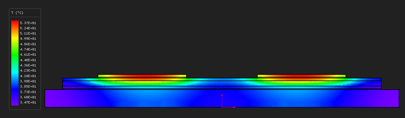
Power-module thermal stack — junction temperature and pulsed loading
Non-machine · Planar thermal, no electromagneticsThe only example in either library with no electromagnetics in it at all: nine layers, all three thermal boundary condition types, and a 10 % duty pulse train whose first peak already lands within 4 K of the final steady state. A module sized on average power is sized wrong.
View exampleGuided case studies
Step-by-step walkthroughs of the GUI workflow on four smaller problems — built by hand rather than by script, and written for someone opening Nabla for the first time.
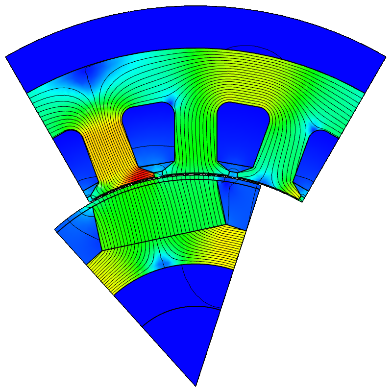
PMSM
Transient 2DCalculate the magnetic field distribution and torque in a permanent magnet synchronous motor (PMSM).
View Example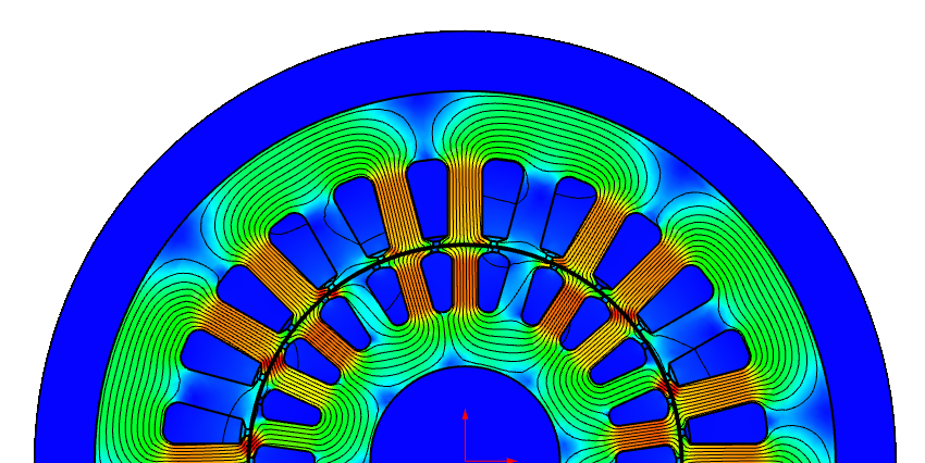
Induction Motor
Transient 2DAnalyze the electromagnetic performance of a squirrel-cage induction motor under various load conditions.
View Example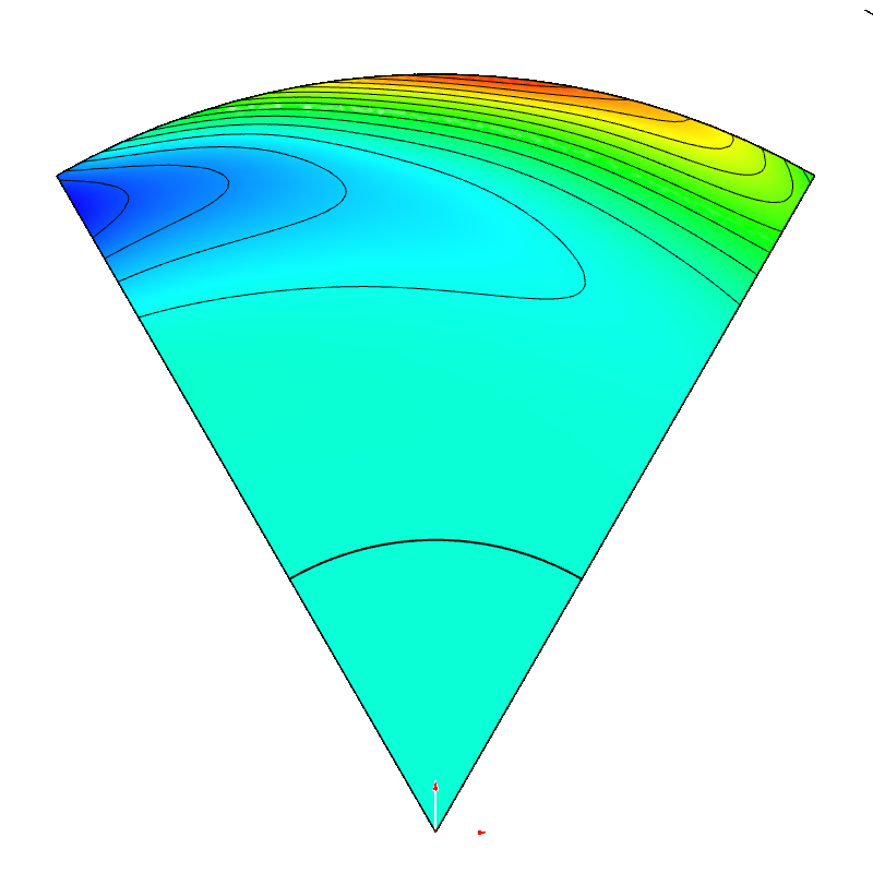
Eddy Current in a Cylinder
Transient 2DSimulate eddy currents induced in a hollow conductive cylinder by a time-varying magnetic field.
View Example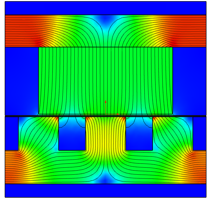
bEMF in Linear Machine
Transient 2DCalculate the back electromotive force (bEMF) in a linear electromagnetic machine during operation.
View Example