Magnetic shield — mu-metal against aluminium, 1 Hz to 100 kHz

← Back to the examples

What you need to run it: the Python API (Automation) plus Core Pro, for the time-harmonic simulation type — which is every solve here. The script says so before it builds anything, and without it still builds, meshes and prints the analytic predictions rather than failing halfway.

What this one is for

Magnetic shielding and conductive shielding are different physics. A high-permeability can shunts flux; that is magnetostatics, so its shielding factor is a number, the same at DC as at 100 kHz. A conducting can shields by induction; it does nothing at DC and its shielding factor rises with frequency. Put both on one axis and the crossover is the whole engineering answer.

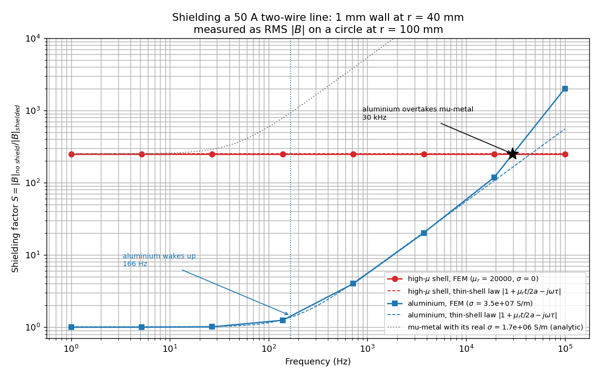
This is also the purest demonstration in the set of what the time-harmonic solver is for: seventeen complex solves on one mesh that never changes, in under three minutes, answering a question every EMC engineer asks and most textbooks answer only in words.

At a glance

Quantity	Value	Unit
Source	two-wire line, Ø4 mm wires 20 mm apart, ±50 A peak	—
Shield	1 mm wall at 40 mm mean radius	—
Legs	no shield / μr = 20 000 / aluminium σ = 3.5e7 S/m	—
Sweep	1 Hz to 100 kHz, 17 points	—
Reference field vs the line-dipole closed form	14.12 vs 14.14 µT, −0.16 (tol 5)	%
High-μ shielding factor	249.7 measured, 244.8 exact, +2.0 (tol 15)	%
High-μ drift across five decades	0.00 (tol 1)	%
Aluminium at 1 Hz	1.000, +0.0 from unity (tol 5)	%
Aluminium corner frequency	166 measured, 181 predicted, −8.3 (tol 25)	%
Crossover	29.7	kHz
Shield Joule loss, 1 Hz to 100 kHz	2.1 µW/m to 0.244 W/m	—
Mesh	50056 nodes, P1	—
Wall time	2 min 45 (1 min 22 coarse)	—

One mesh, three materials

All three legs share one mesh, node for node, differing only in the two numbers written into the Shield region:

Leg	μr	σ (S/m)
reference (“no shield”)	1	0
ferromagnetic	20 000	0
conductive	1	3.5e7

That is deliberate, and it is the method. Region properties are read when the solver input is written, which happens inside the solve, so changing them after meshing needs no remesh. The shielding factor is a ratio, and a ratio taken across two different meshes measures the meshes as much as the physics.

What the sweep measures

S = |B|unshielded / |B|shielded, from the RMS of |B| over one period at eight points on a circle 100 mm out. Two details there are load-bearing.

A time-harmonic solution is a phasor. A point probe reads one reconstructed snapshot, which is one instant of a vector that in general traces an ellipse. A single step is not a shielding measurement; the RMS over a whole period is.

A run asked for N snapshots per period hands back N+1. The last is t = T, the same phase as t = 0. Averaging over all of them counts that phase twice, which biases the RMS by about 2 % here — and not equally in the two legs, because the eddy-shielded field is phase-shifted with respect to the source and so gets sampled differently. The script takes one period and no more.

The eight angles are measured separately and only then averaged, because their spread is a check in its own right: the exterior field of this device is a single dipole mode, so a shell must attenuate it by the same factor everywhere on the circle. It does, to 1.3 % for the high-μ can and 4.3 % for the aluminium one.

The checks

1. The reference is the closed-form line dipole. Two antiparallel line currents a distance d apart give a field of magnitude μ0·I·d/(2πr²), independent of angle. Measured 14.12 µT RMS against 14.14 µT analytic, −0.16 %. Everything else on this page is divided by that number, so it is the first thing to check.

2. The high-μ shell against the exact concentric-shell result. For a shell of relative permeability μ between radii a1 < a2, the dipole-mode exterior amplitude is reduced by

S = [ (mu+1)^2 - (mu-1)^2 * (a1/a2)^2 ] / (4 mu)

which is 244.8 here. The familiar thin-wall form 1 + μrt/(2a) gives 251.0 — 2.5 % apart at this permeability, which is why the anchor is the exact one. Measured 249.7, +2.0 %.

3. The high-μ shell has no frequency scale. With σ = 0 the mass matrix is empty and (K + jωM)Â = F̂ is the static problem at every frequency. Measured drift across five decades: 0.00 %. It is an easy check and a real one — it says the time-harmonic path reduces to the static one exactly.

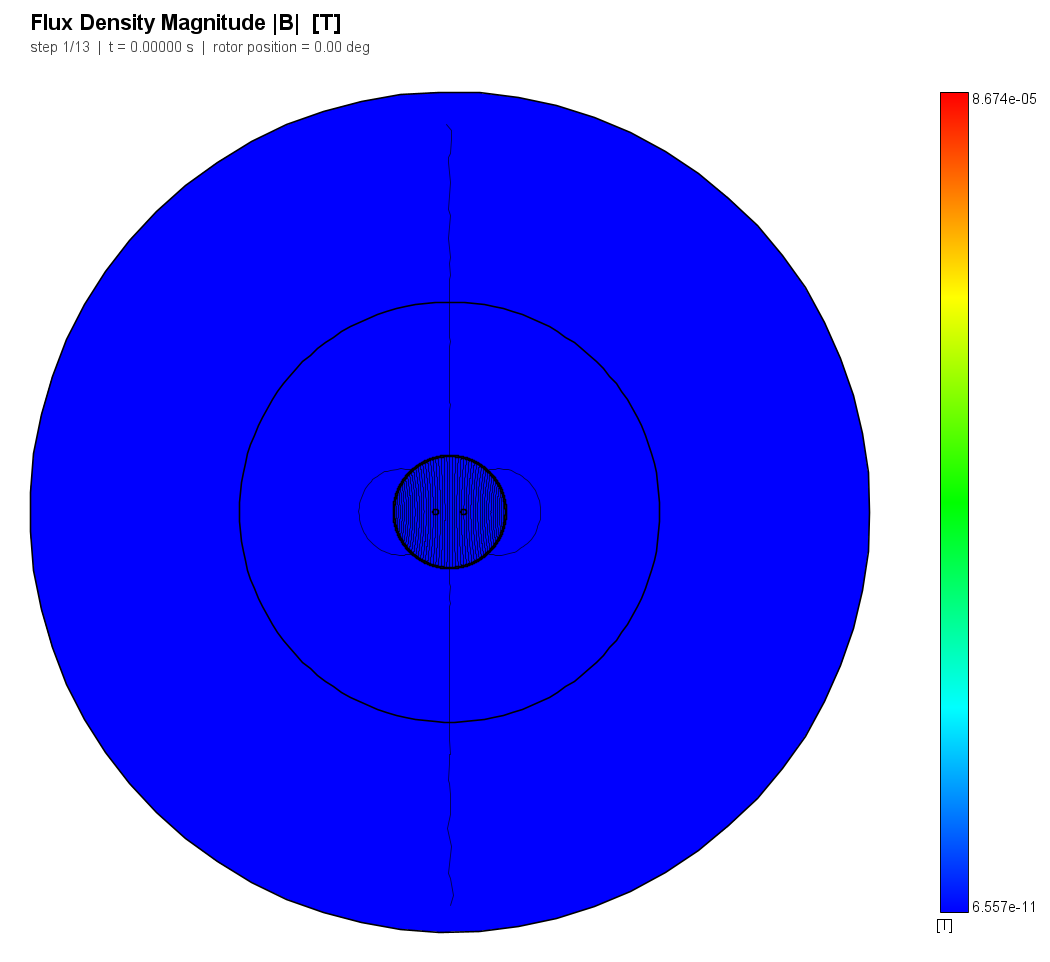
4. The aluminium can does nothing at DC. S = 1.000 at 1 Hz.

5. The aluminium corner frequency. For a thin conducting shell with a dipole source inside, S = |1 − jωτ| with τ = μ0σta/2 — here 0.880 ms, so S = √2 at 181 Hz. Log-interpolated from the sweep: 166 Hz, −8.3 %.

A deliberate departure. The obvious check would be the crossover against “skin depth equals wall thickness”. That is the wrong scale for a thin shell: eddy shielding starts when the shell's own L/R time meets the period (181 Hz here), long before the wall is a skin depth thick (7.2 kHz). The example checks the scale that actually governs the corner and reports the other frequency separately, as the onset of the exponential regime — which is exactly what the figure shows the FEM curve doing when it lifts above the dashed thin-shell line above about 10 kHz.

The headline

Above 29.7 kHz a 1 mm aluminium can out-shields a 1 mm mu-metal one — and it costs nothing, does not need annealing, and does not care about being dropped. The thin-shell laws put that crossing at 45 kHz; the FEM puts it lower because by then the wall is two to four skin depths thick and the can has stopped shielding as ωτ and started shielding exponentially.

The price is dissipation, because shielding by induction is shielding by dissipation: the shield's Joule loss runs from 2.1 µW/m at 1 Hz to 0.244 W/m at 100 kHz. The high-μ shell dissipates nothing at all, at any frequency, by construction.

Caveats, stated rather than tuned away

• The ferromagnetic leg is solved with σ = 0. That buys the figure its cleanest statement — the red curve is the pure flux-shunting mechanism, with no frequency scale of its own — and it is a fair model of a laminated or insulated high-permeability shell. A real solid mu-metal can has σ ≈ 1.7e6 S/m, and because its eddy term carries μ_r too, its corner sits near 0.2 Hz: below the bottom of this sweep. Its curve is on the figure as the grey dotted line — analytic only, nothing is solved with it. Adding it as a third solved leg costs one more entry in a list and eight more solves.
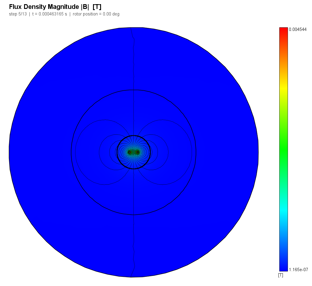
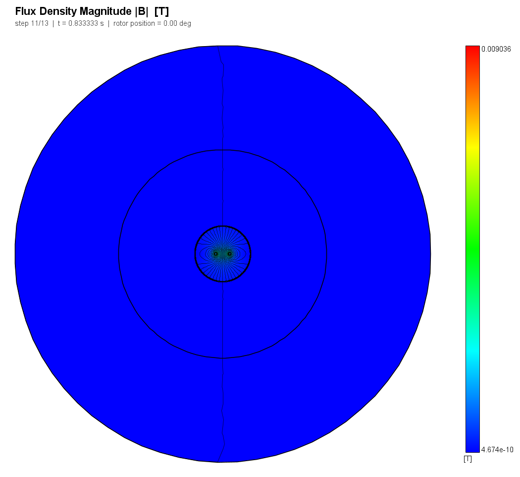
• The material is linear. Real mu-metal saturates around 0.7 T, and the peak |B| anywhere in this model is 9 mT — at the conductor surfaces, where the shield is not. So the assumption is safe here and would not be in a shield carrying real flux, and nothing in the script checks it for you: raise the line current far enough and it will keep reporting a shielding factor that no longer exists.
• The top of the aluminium leg is the mesh-sensitive point. At 100 kHz the skin depth in aluminium is 0.27 mm and the wall is 3.7 of them. Refining the shield mesh from 50 056 to 127 156 nodes moves S at 100 kHz by +2.5 % and the shield loss by +7.4 %; every other point moves under 1 %.

A trap this example walked into

A circle is a polygon in the mesher's input, and how fine a polygon is decided before there is a mesh to ask — it falls back to the global default mesh size when no region triangulation covers the circle yet. On this model that default gave the shield wall nine segments. Nine segments at 40 mm radius is a 2.4 mm sagitta: the two walls of a 1 mm can cross each other, the annulus is never a closed face, and the mesher floods the air region's material straight through it.

Nabla's rule M18 caught it exactly as designed, naming both the region and the region that ate it:

M18: region 'Shield' has no mesh elements. ... Region 'AirNear' owns the elements
around that point (4788 of them), so that is where it leaked to. As meshed,
'Shield' would solve as the material of 'AirNear'.

The fix is two explicit subdivision calls, and any thin annular feature drawn from circles needs them.

Running it

python magnetic_shield.py                    # both legs + reference, ~2 min 45 s
python magnetic_shield.py --coarse           # every mesh area x4, ~1 min 20 s
python magnetic_shield.py --stage conductive # one shield only

--coarse turns the recorded baselines off, because a quarter of the mesh legitimately moves the top aluminium point; the physics anchors still run.

Try this next

• Add the solid mu-metal leg that is currently only a dotted analytic line. It is one entry in the material list, and its corner near 0.2 Hz is the reason a real can behaves like neither of the two idealised legs.
• Move the crossover. Wall thickness, shield radius and conductivity all enter the corner frequency, and the two analytic laws on the figure are computed from those constants — so the checks follow the device rather than being pinned to it.
• Push the top frequency up, and raise the shield mesh resolution with it: the requirement is a few elements across the skin depth.

About these numbers

This is a demonstration shield, not a product specification. Every figure on this page came out of the run described here at the settings the script ships with. For accuracy against a stated reference and tolerance, the validation dossier is where that question belongs.