E04 — 24-slot / 8-pole V-shape interior-PM synchronous machine
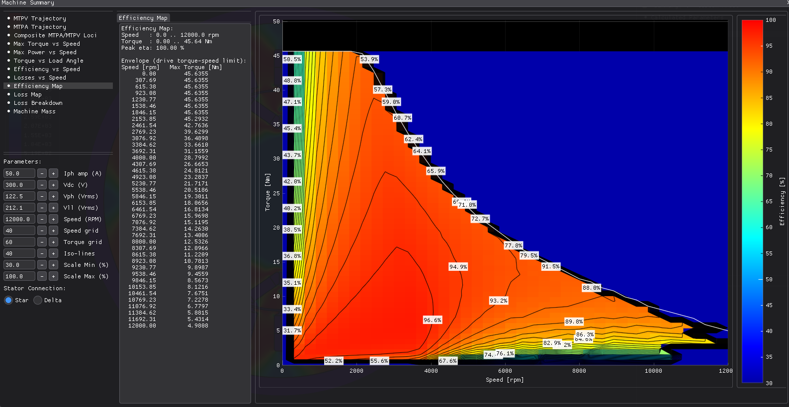
PMSM · Custom Rotor (DXF, V-shape IPM) · 24 slots / 8 poles · 45.903 N·m at 3000 rpm · 94.2 % efficient · 8156 nodes · 85 s
What you need to run it: the Python API and the Machines module. Opening the model and reading results that are already there never requires a licence.
At a glance
| Quantity | Value | Unit |
|---|---|---|
| Speed | 3000 | rpm |
| Electrical frequency | 200.0 | Hz |
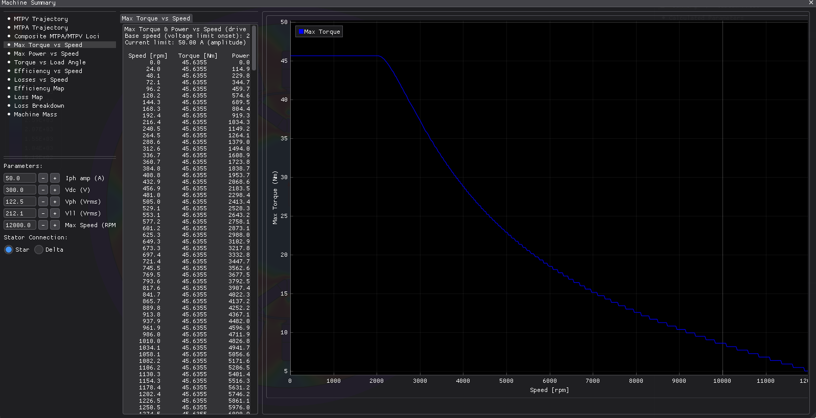
| Average torque | 45.903 | N·m |
| Torque ripple | 38.3 | % |
| Cogging torque, peak-peak | 0.327 | N·m |
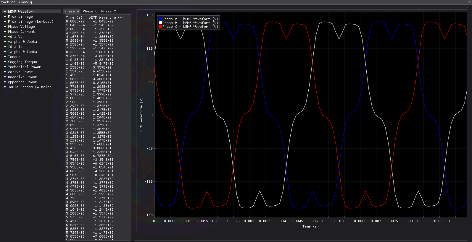
| Back-EMF, RMS | 107.3 | V |
| Mechanical power | 14.421 | kW |
| Efficiency | 94.15 | % |
| Power factor | 0.812 | — |
| Total losses | 895.2 | W |
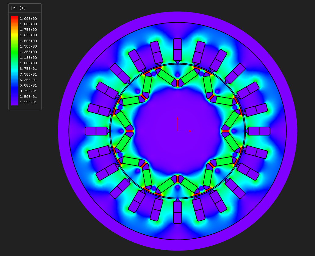
| Max B, stator tooth | 1.531 | T |
| Mesh | 8156 nodes, 15939 elements, P1 | — |
| Wall time, end to end | 85 | s |
A 15 kW traction-style motor with the magnets buried in a V under each pole. Open this one if you want to see reluctance torque doing real work — a third of the output here — or if you want to draw your own rotor rather than pick one from the list.
The rotor is a DXF. The script draws it, imports it and then places a region on each feature: lamination, two magnets, the flux barriers. Nothing is created for you, not even the rotor iron. That is the whole custom-rotor route, and it is currently the only way to get a buried magnet out of Nabla.
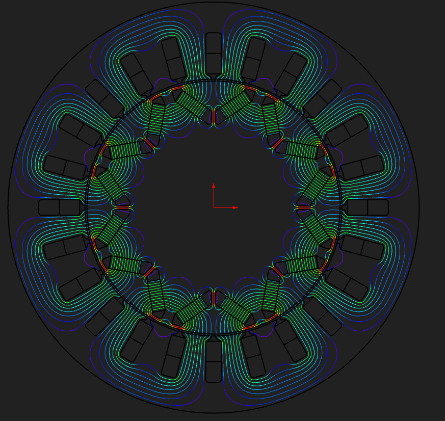
One pole is solved — three slots over 45°, closed anti-periodically.
The design
| Layer | Radii (mm) | Set by |
|---|---|---|
| rotor | 0.0 → 49.25 | solid lamination to the axis, see below |
| centre bridge | 0.0 → 0.75 | centreBridgeHalf, the d-axis iron the barriers stop on |
| V vertex | 34.000 | vertexRadius, where the two arms meet |
| magnet corners | 34.9 → 47.1 | 5 mm thick, 12 mm long, on a 110° V |
| barrier tips | → 48.05 | bridge, 1.2 mm under the rotor surface |
| air gap | 49.25 → 50.0 | airGap 0.75 |
| stator bore | 50.000 | ID 100 |
| slot bottom | 68.000 | slotDepth 18, slotWidth 6 |
| stator OD | 80.000 | OD 160, back iron 12 |
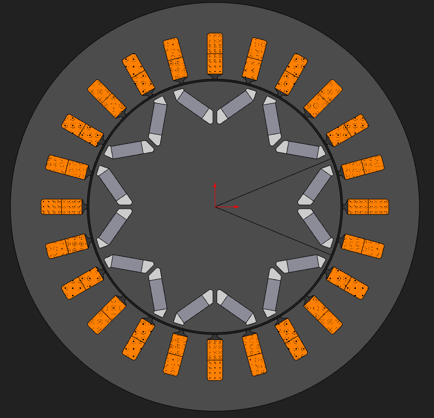
Trapezoidal teeth, 80 mm axial length, four pole pairs, distributed full-pitch winding.
The rotor drawing
One pole, drawn about the +x axis: twenty lines and eight arcs, generated from ten numbers in
the script's VPOLE dictionary. The V is specified the way a V-IPM usually is, by the opening
angle between the arms measured at the vertex, opening towards the air gap. It is 110° here.
The Prius uses 145° on the same pole count.
Two details follow from that angle rather than being chosen:
The end barriers run radially out to the bridge, not along the magnet axis. At 110° each arm points 55° away from the d-axis, so a barrier continuing along the magnet would hit the pole edge long before it reached the surface.
The magnets are short — 12 mm on a 38.7 mm pole arc. The arms cross the 45° pole wedge quickly, and what limits their length is the q-axis rib at one end and the 1.2 mm surface bridge at the other.
Change VPOLE and the drawing follows: corner radii, tangent points, arc angles, region seeds
and magnetisation directions are all derived from those ten numbers, so changing the V angle
is one edit.
The .dxf is an output, not an input. It is regenerated on every run, so editing it by
hand and re-running throws the edit away. Change VPOLE instead, or pass --keep-dxf to
import the drawing on disk unchanged — but read that flag's warning first, because region
seeds and magnetisation directions do not follow a hand-edited drawing.
Why the rotor has no bore
The rotor is solid steel all the way to the axis, which looks wasteful and is deliberate.
The machine module draws two radial segments from the axis to close the sector, and it does not split them where your drawing happens to touch. An imported entity that ends part-way along one of those segments makes a T-junction, the polygon description cracks, and a neighbouring region floods across the crack. A bore drawn as an arc across the pole pitch is exactly that case.
The failure is silent. The model meshes, the band check passes, the solver converges, the field plot looks normal, and only the flux is wrong — 2.6 times low when this bit a real design. Keep every drawn feature clear of the sector edges, and if you need a bore, put it in as part of the same drawing rather than crossing the seams.
The script checks the mesh for the defect anyway rather than trusting the drawing: every region seed has to own elements, and a permeability probe in the lamination has to read steel rather than air.
Winding and materials
| Stator and rotor core | M-19 Steel, nonlinear BH |
| Magnets | N35SH, chosen because it carries a demagnetisation curve |
| Magnet conductivity | 6.7 × 10⁵ S/m (sintered NdFeB), for the eddy currents |
| Magnetisation | ±35° from the d-axis, perpendicular to each arm |
| Flux barriers | air |
| Winding | distributed double layer, q = 1, full pitch |
| Turns per coil | 10, one parallel branch |
| Slot fill | 0.45 |
| End winding | 12 mm extension, resistance and inductance included |
The magnet grade matters for more than temperature here. The demagnetisation-risk field needs a material that carries a demagnetisation curve, and not every magnet in the library does.
Operating point
| Current | 50 A peak at 30° current angle, so I_d = −25 A, I_q = 43.3 A |
| Speed | 3000 rpm, so 200 Hz electrical |
| Window solved | two electrical periods, 48 steps each |
| Eddy currents | on, in the magnets |
| Mesh | 1.2 mm default; 0.5 mm in the rotor core, 0.8 mm in magnets and barriers |
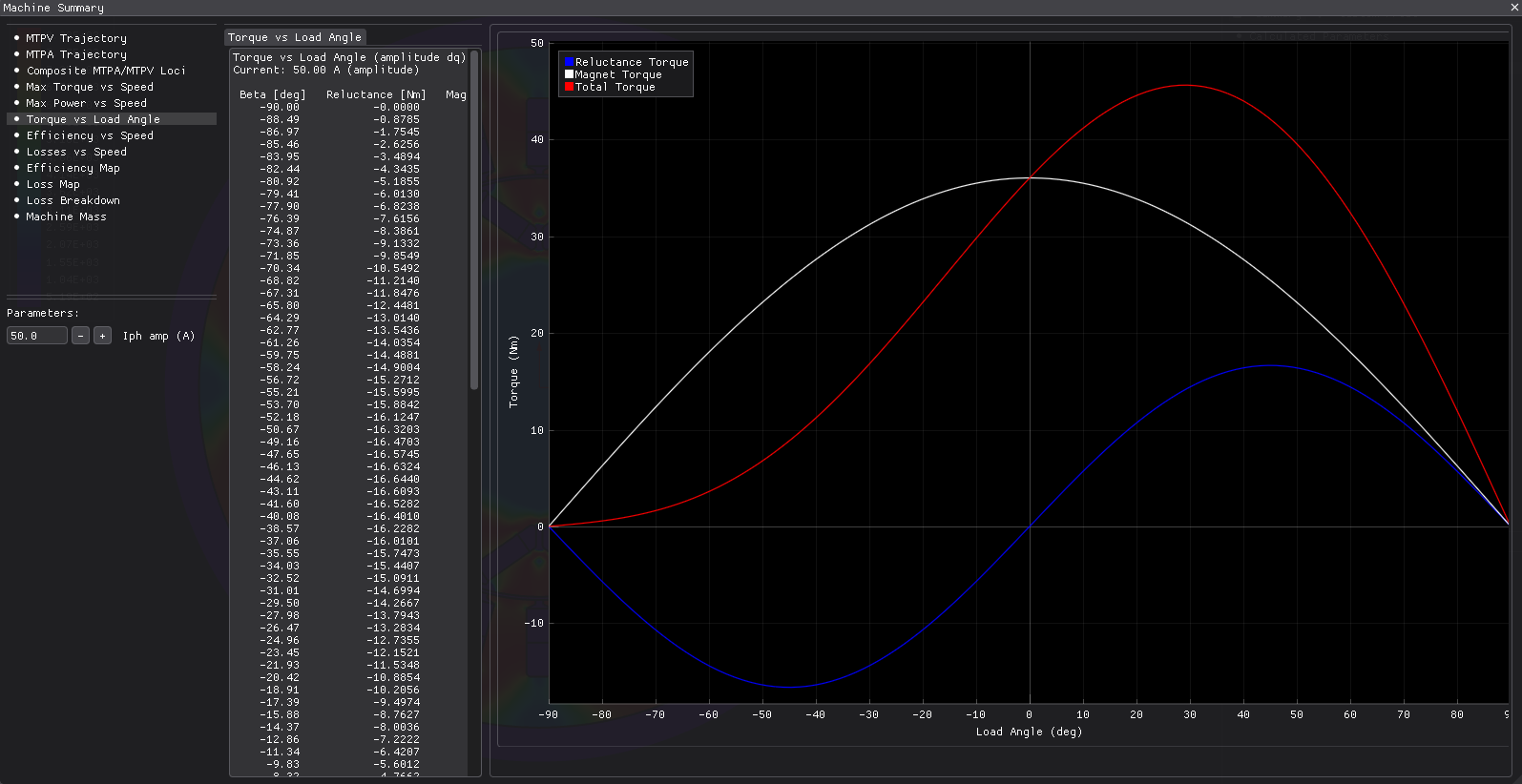
The current angle is the point of the machine. A negative d-axis current is what turns saliency into torque; at I_d = 0 an IPM gives you its magnet torque and nothing else.
Two periods rather than one, because of the eddy currents. With eddy currents on, the transient is a genuine diffusion problem starting from zero field, so the first steps carry a startup transient with almost no torque. That is physics, not a defect, but it is not the steady state you want summarised. The summary reduces the last electrical period, so a second period is enough to leave the startup behind. Summarising the first period instead put the torque ripple at 122 % of the mean and the power balance 24 % out; at two periods they read 38 % and 0.2 %.
Running it
Open pmsm_ipm_v_shape.nbl and press Solve — about a minute. The model ships; the solved field
does not, because it is a 30 MB file.
From Python:
python build_pmsm_ipm_v_shape.py             # build, solve, render, report
python build_pmsm_ipm_v_shape.py --no-solve  # geometry and mesh only, about 15 s
python build_pmsm_ipm_v_shape.py --no-eddy   # without the magnet eddy currents
python build_pmsm_ipm_v_shape.py --keep-dxf  # import the .dxf on disk as it stands
What to look at
The torque split. This is why the example exists. Put the solved inductances and magnet flux into the dq torque equation:
T = 1.5 · p · [ λ_pm · I_q + (L_d − L_q) · I_d · I_q ]
  = 29.8 (magnet) + 14.4 (reluctance) = 44.2 N·m
against 45.9 N·m from the field solution, so the dq model accounts for 96 % of it, and a third of the torque is reluctance. Compare that with E02, where a spoke rotor with a similar saliency ratio gets only 2.5 % from the reluctance term — the difference is the current angle and where the saliency sits.
One trap in that arithmetic: the inductances come back in microhenry, not henry.
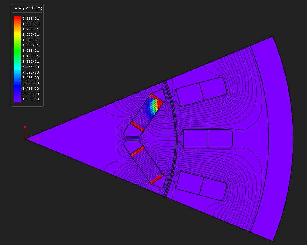
Demagnetisation risk. demag_risk.png shows the field, and it reads a few per cent at the
magnet centres at this operating point. The number is a percentage of the way from the working
point towards the knee of the demagnetisation curve at the material's hottest published curve,
so 0 % is comfortable and 100 % is the knee. Watch the corners of the magnets nearest the
barriers — that is where a real IPM demagnetises first.
Saliency. L_q / L_d is 2.22. Both come from small test currents applied on top of the magnet state, so they include stator saturation, not just the rotor geometry.
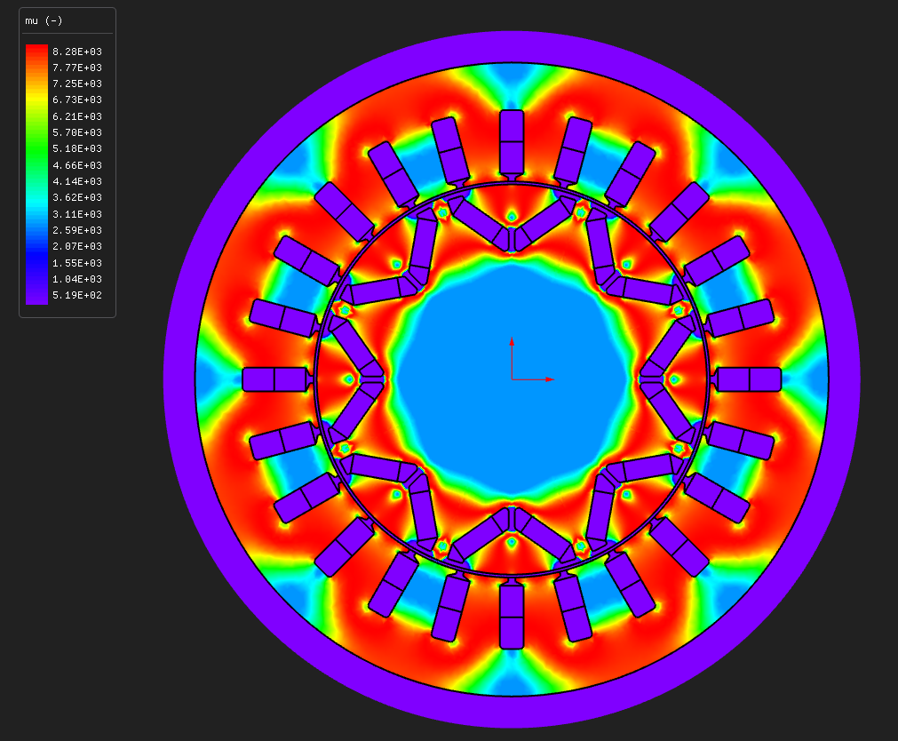
The region map. region_map_mu.png colours the model by permeability, which is the quickest
way to confirm that steel is steel, magnet is magnet and the barriers really are air. On a drawn
rotor that is worth a look before you trust anything else.
Torque ripple is high — 38 % — and it is the design. One slot per pole per phase, a flat-topped pole and no skew leave nothing to suppress the slot harmonic. Skew is the usual answer; E03 shows what it buys.
Try this next
openingAngleDeg, 110° towards 145° — the arms turn more tangential, the magnets can grow, and the machine trades saliency for magnet torque.centreBridgeHalf, 0.75 → 1.5 mm — a wider centre bridge is mechanically stronger and magnetically worse. It short-circuits more magnet flux, and back-EMF and magnet torque fall with it.--no-eddy— run it against the base case to see what the solid magnets cost. One period is enough without them.- Sweep the current angle from 0° to 45° to trace this rotor's own MTPA curve. At 0° the reluctance term disappears entirely.
About these numbers
The dimensions are invented but plausible. This is not a copy of a published design and no measurement backs it. The validated V-magnet IPM is the 2004 Toyota Prius traction motor, and that is the one to cite for an IPM accuracy claim — see the validation dossier.
The rotor iron loss reads zero here. That is because a region you seed yourself starts with zero Steinmetz coefficients and the loss terms multiply by them, so switching iron loss on is not enough on its own. E06 shows how to copy the coefficients onto a drawn region, and what the answer looks like once you have.
More from this run