E02 — 36-slot / 6-pole spoke-type PM synchronous machine

← Back to the examples

What you need to run it: the Python API, the Machines module, Performance analysis and Materials Pro. Opening the model and reading results that are already there never requires a licence. Performance analysis covers the maps, the MTPA trajectory and the pies; Materials Pro covers the iron-loss fit. Without them the machine still builds and solves - it is the analysis that stops.

At a glance

Quantity	Value	Unit
Speed	1500	rpm
Electrical frequency	75.0	Hz
Average torque	31.534	N·m
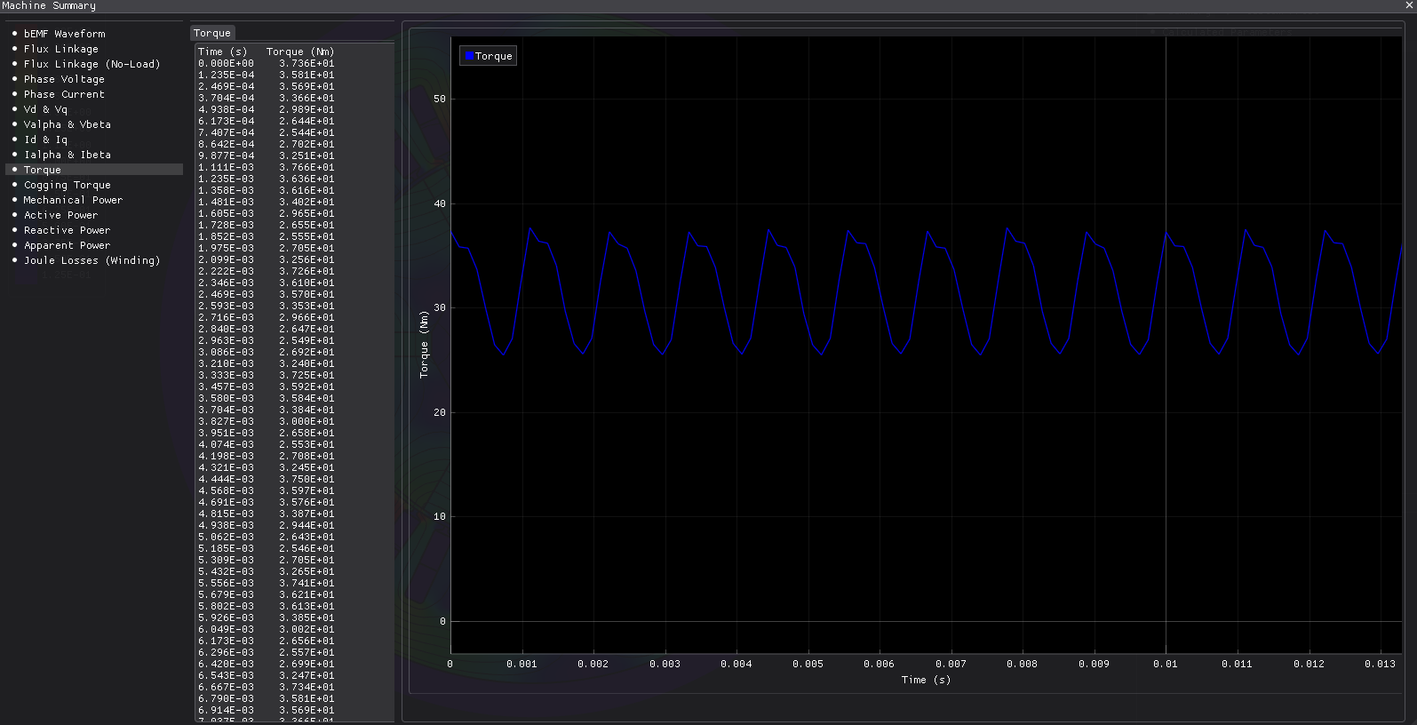
Torque ripple	37.3	%
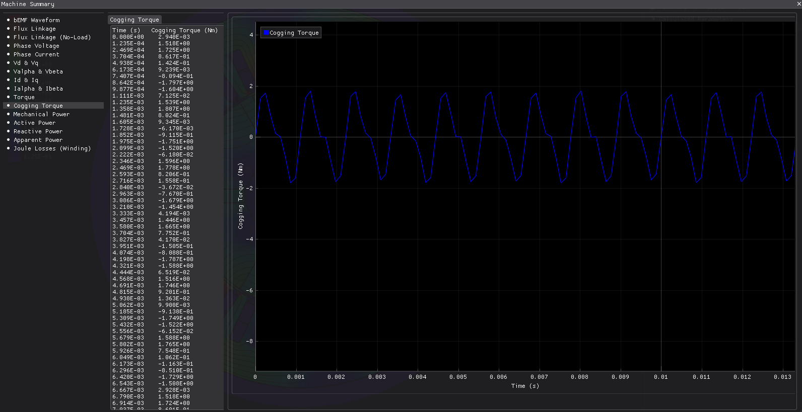
Cogging torque, peak-peak	3.282	N·m
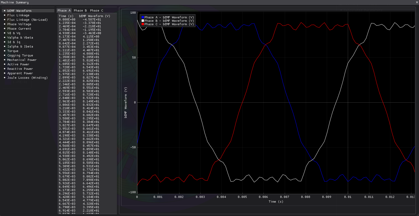
Back-EMF, RMS	71.5	V
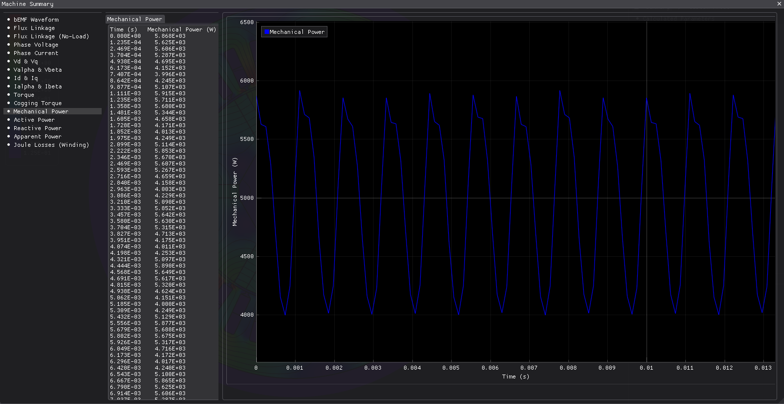
Mechanical power	4.953	kW
Efficiency	95.51	%
Power factor	0.959	—
Total losses	232.7	W
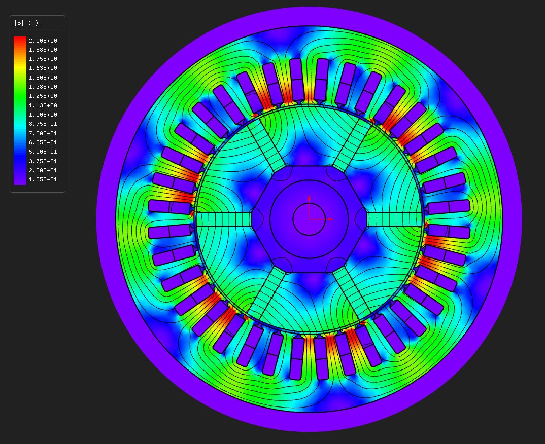
Max B, stator tooth	1.733	T
Mesh	5182 nodes, 9940 elements, P1	—
Wall time, end to end	103	s

A 5 kW spoke-rotor machine, and the one to open when you want the dq performance work: saliency, an MTPA current angle, an efficiency map, a loss map and a mass breakdown.

The magnets stand radially between iron pole pieces instead of lying on the surface. Flux from two magnet faces feeds one pole arc, which concentrates it, and the two axes stop looking alike: the d-axis path runs through the magnets, which are magnetically about as good as air, while the q-axis path runs through solid iron. L_q comes out around 1.6 times L_d, so the current angle becomes something to choose rather than something to leave at zero.

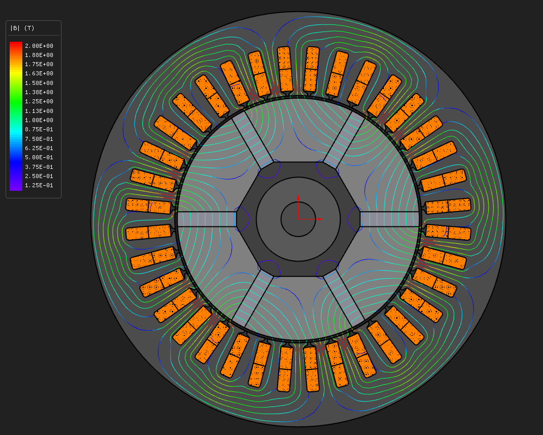
One pole is solved — six slots over 60°, closed anti-periodically.

The design

Layer	Radii (mm)	Set by
shaft bore	7.000	shaftThickness 10 (a 14 mm bore)
rotor shaft	7.0 → 17.0
rotor hub, non-magnetic	17.0 → 25.0	coreThickness 8
magnet and pole piece	25.0 → 49.0	PMThickness 24 radial, PMWidth 6 tangential
air gap	49.0 → 50.0	airGap 1
stator bore	50.000	ID 100
slot bottom	70.000	slotDepth 20, slotWidth 5, slotOpening 0.25
stator OD	84.000	OD 168, back iron 14

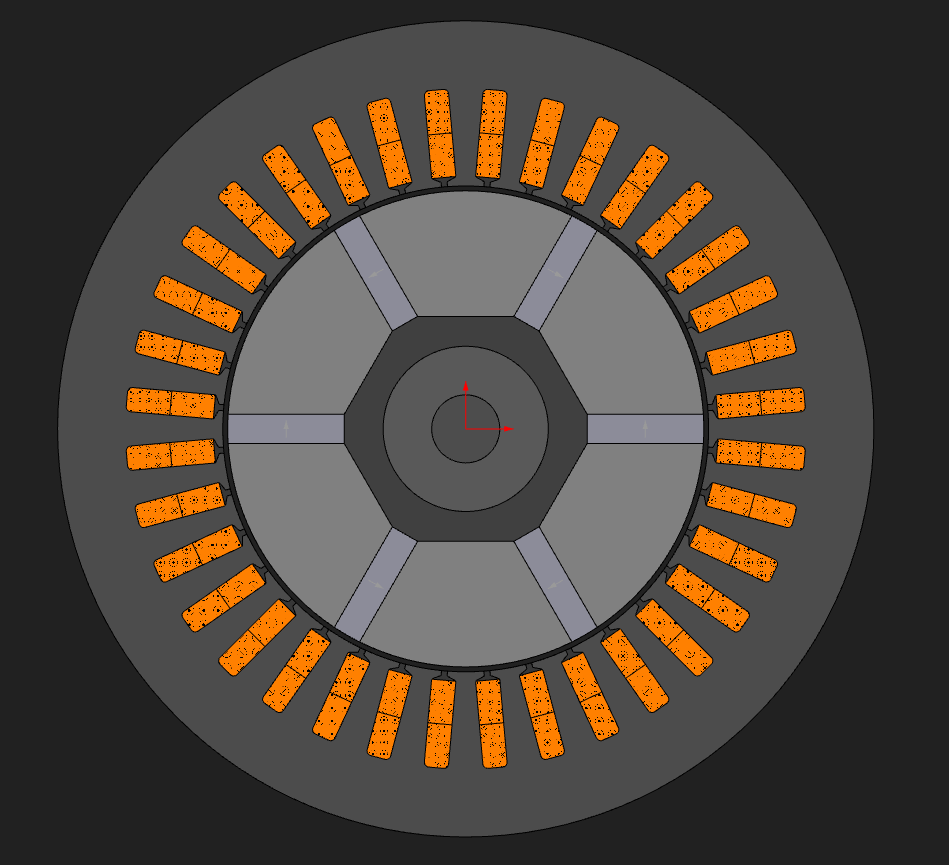
Trapezoidal teeth, 100 mm axial length, three pole pairs.

On a spoke rotor PMThickness is the magnet's radial length and PMWidth its tangential thickness. That is the opposite of a surface-magnet rotor, where the magnet lies along the gap, and it is what buys the flux concentration: two 24 mm magnet faces feed a 51 mm pole arc.

Two region names that do not mean what they say

This is the part of a spoke rotor that is easiest to get wrong, and both mistakes are quiet ones — the model still solves and still looks like a motor.

PMSpacer* regions are the iron pole pieces, not spacer air. They carry the whole airgap flux, so give them your core steel and your loss coefficients.

Rotor Core is the non-magnetic hub. The template leaves it at µ_r = 1 deliberately and this model leaves it alone. Assign a soft-magnetic material to it and you short-circuit every magnet through the hub. The solve converges, the field plot still looks reasonable, and most of your back-EMF is simply missing.

The same naming catches two summary rows. IronLossesRotor and MaxFluxDensityRotor are both computed on the region called Rotor Core, which here is that inert hub, so they read close to zero and tell you nothing about the rotor. Read the pole pieces directly instead — ask for Iron AC Losses Total on the PMSpacer* regions and scale by the number of symmetry sectors. Done that way the pole-piece iron loss is about 0.17 W, which is a small number you can believe rather than a small number you were handed by accident. In the mass pie the pole pieces land in the "Sleeves / Wedges / Spacers" slice for the same naming reason.

Winding and materials

Stator core and rotor pole pieces	M-19 Steel, nonlinear BH
Rotor hub	left non-magnetic, see above
Rotor shaft	1020_steel
Magnets	N42
Winding	distributed, double layer, 36 coils, 2 parallel branches
Turns per coil	10
Coil pitch	5 slots of 6, giving a winding factor of 0.933
Slot fill	0.45
End winding	15 mm extension, resistance and inductance included

The 5/6 pitch is doing real work. A spoke rotor's airgap flux is close to a square wave, so its 5th and 7th harmonics are large, and those are what drive 6th-harmonic torque ripple. Chording to 5/6 knocks both down to a quarter for 3.4 % of the fundamental. On this design it took back-EMF distortion from 22.5 % to 17.1 % and torque ripple from 71 % to 46 %.

Operating point

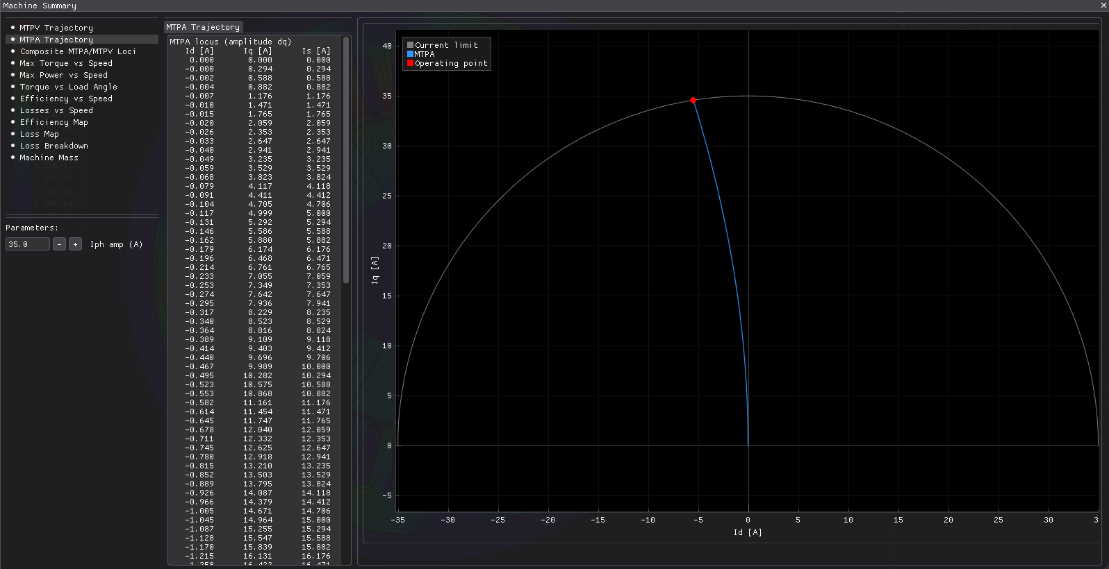
Current	35 A peak, 9° ahead of the q-axis (I_d = −5.5 A, I_q = 34.6 A)
Speed	1500 rpm, so 75 Hz electrical
Window solved	one electrical period, 108 steps
Mesh	0.9 mm maximum, about 5 200 nodes
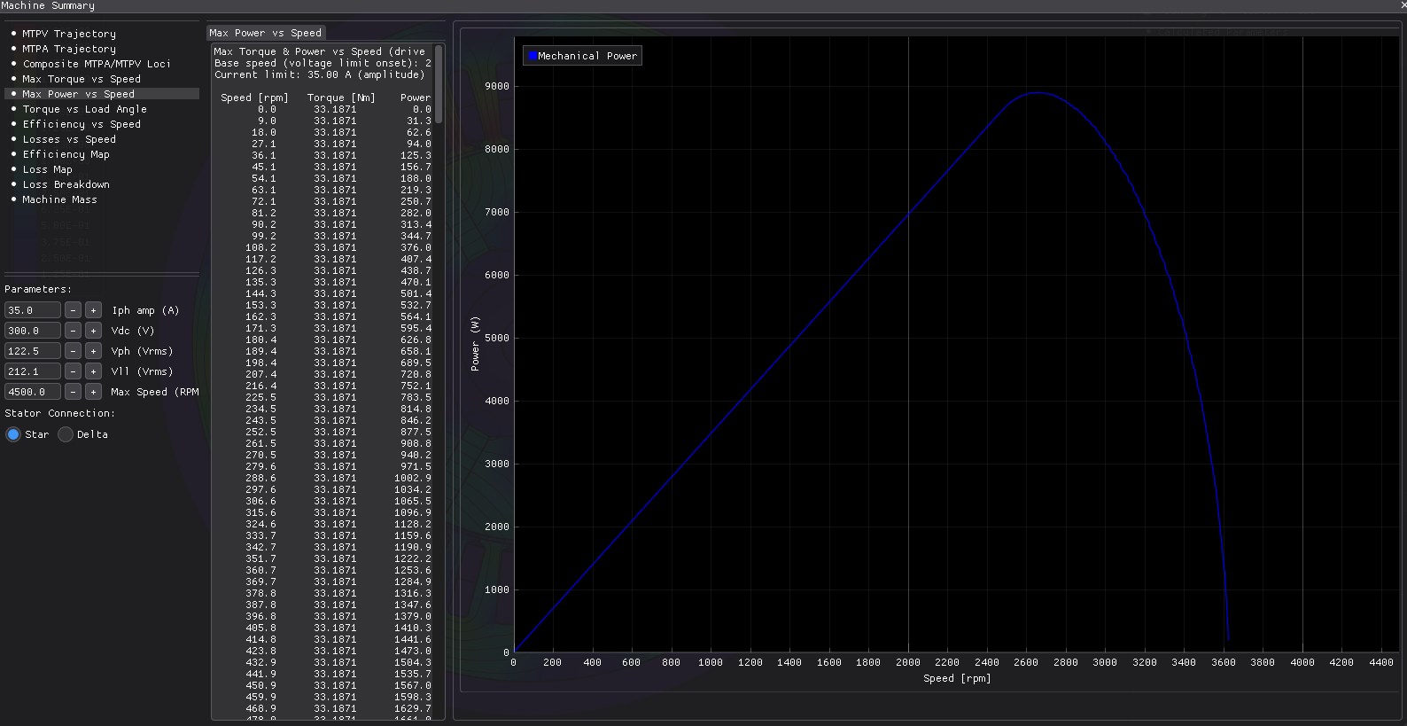
Drive assumed for the maps	400 V DC, 35 A phase limit, swept to 4800 rpm

That 9° is the closed-form MTPA angle for the extracted parameters, and the performance analysis finds the same locus independently. The two agree to a twentieth of a degree, which is a good check that the extracted L_d, L_q and magnet flux describe the machine you solved.

108 steps rather than 36, for a specific reason. Chording removed the 6th-harmonic ripple, which leaves the slot harmonic — twelve cycles per electrical period on this machine — as the biggest component left. Thirty-six steps gives three samples per cycle and reports 55 % ripple, which is an aliasing artefact. A hundred and eight steps gives nine samples and reports 37 %, which is the machine.

Running it

Open pmsm_36s6p_inset.nbl and press Solve. The solved field is not shipped with this one — it is a 41 MB file that regenerates in a couple of minutes — so opening the model shows you the geometry and the settings, and the field appears once you solve.

From Python:

python build_pmsm_36s6p_inset.py                  # build, solve, analyse, report
python build_pmsm_36s6p_inset.py --no-performance # skip the loci and the maps
python build_pmsm_36s6p_inset.py --no-solve       # geometry and mesh only

Budget about three minutes for the full run. Roughly half of that is the performance analysis rather than the field solve.

What to look at

Saliency and where the torque comes from. L_q / L_d is 1.61. Put the extracted parameters into the dq torque equation and you get 32.3 N·m of magnet torque against 0.84 N·m of reluctance torque — about 2.5 % of the total. That is what a spoke rotor is. It is a flux-concentrating magnet machine that happens to be salient, not a reluctance machine. For the case where reluctance is a third of the torque, see E04.

Note that the summary reports SaliencyRatio as L_d / L_q, which is 0.62 here — the reciprocal of the 1.61 quoted above. Both conventions are in circulation, so check which one you are reading before you compare against a datasheet.

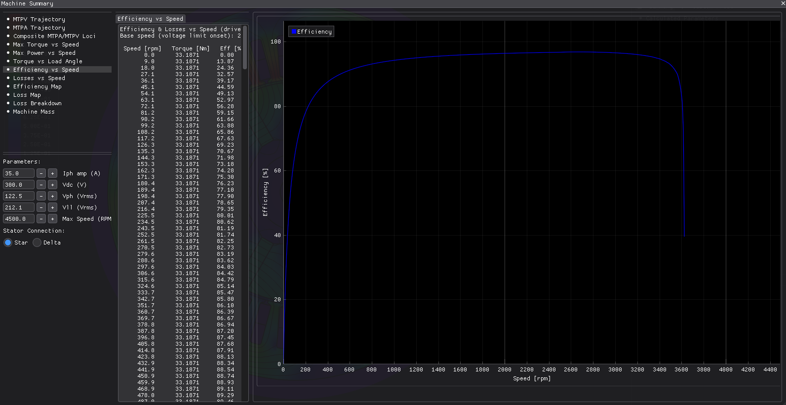
The maps. efficiency_map.csv and loss_map.csv carry the full sweeps, and the PDF report draws them. Peak efficiency on the map is about 97 %, against 95.5 % at the rated point.

No MTPV locus, and that is correct. Maximum torque per volt only exists when the characteristic current — magnet flux divided by L_d — falls inside the current limit. Here it is 128 A against a 35 A limit, so this design cannot be flux-weakened towards infinite speed. It runs out of torque instead, at about 4870 rpm on the envelope. If the API tells you the dq parameters have not been extracted, ignore the wording: they were extracted, and they are exactly what rules the locus out.

Fitted iron loss. No shipped material carries a specific-loss table, so this example brings its own — 48 points of loss against frequency and flux density, representative of a 0.35 mm non-oriented grade at about 2.6 W/kg for 50 Hz and 1.5 T. It is generated from a known Steinmetz triple, which means the fit can be checked against the answer it should return, and it returns it. Use the same route for your own steel: fitIronLossCoefficients against a table of measured points, then assign the coefficients to the region.

Where the ripple comes from

Thirty-seven per cent torque ripple is what this rotor gives, not a modelling artefact. A spoke rotor with rectangular pole pieces and no surface shaping produces a nearly square airgap flux wave, and the parametric builder offers no pole-shoe shaping to soften it. Chording already removed the part driven by the 5th and 7th harmonics; what remains is the slot harmonic, and the fix for that is skew, which this machine does not use.

Here is the trade across the two levers that are available, all at 108 steps:

air gap	slot opening	coil pitch	T_avg	ripple	bEMF THD	L_q/L_d
0.6	0.40	6/6	34.2	70.7 %	22.5 %	2.16
1.0	0.25	6/6	32.6	46.5 %	23.5 %	1.55
0.6	0.25	5/6	35.1	54.0 %	20.6 %	1.91
1.0	0.40	5/6	31.2	45.9 %	17.2 %	1.56
1.0	0.25	5/6	31.5	37.3 %	17.1 %	1.61

The shipped design is the last row. Opening the air gap from 0.6 to 1.0 mm is what costs the saliency, and it is also what buys most of the ripple reduction.

Try this next

• --no-performance — roughly halves the wall time when you only want the field solution.
• --steps 36 — watch the reported ripple climb to about 55 % for no physical reason. It is worth doing once, so you recognise the effect when you meet it in your own model.
• Thin the magnets. PMThickness from 24 mm down towards 16 gives less flux concentration and less torque, and a higher saliency ratio, because L_d rises as the magnetic gap shortens.
• Add stator skew with setMachineGeometry("stator", "skewAngle", …) and more than one slice. It is the classical fix for both the cogging and the slot-harmonic ripple. E03 is built around it.

About these numbers

The dimensions are invented but plausible. This is not a copy of a published design and no measurement backs it, so please do not quote it as evidence of accuracy. For that, see the validation dossier.

More from this run