Power-module thermal stack — steady state, pulsed transient and a ceramic swap

← Back to the examples

What you need to run it: the Python API (Automation) and the Thermal module. Nothing else — no Core Pro, no Machines. Without the thermal module the script says so before building anything and still produces the geometry and the mesh; opening the committed model and reading its committed solution is never gated.

What this one is for

This is the thermal demo, and the only example in either library with no electromagnetics in it at all: the heat sources are given, the unknown is temperature, and the thermal module is the whole of it. If you came to Nabla for conduction rather than for fields, this is the page that shows what that looks like end to end.

The device is a two-die power module in cross-section, on a directly liquid-cooled baseplate — a traction-inverter stack, in the layer order a real one has.

The stack

Layer (bottom to top)	Thickness	Width	Material	k (W/mK)
Copper baseplate	2.0 mm	40 mm	copper	400
Baseplate solder	0.1 mm	36 mm	SAC305	58
DBC copper, bottom	0.3 mm	36 mm	copper	400
DBC ceramic	0.6 mm	36 mm	Al2O3	24
DBC copper, top	0.3 mm	36 mm	copper	400
Die attach ×2	0.1 mm	10 mm each	SAC305	58
Silicon die ×2	0.3 mm	10 mm each	silicon	148

The stack is 3.7 mm tall, 40 mm wide and 20 mm deep, the two dies are 8 mm apart edge to edge, and each dissipates 100 W. The baseplate underside is cooled by a convection film at 15 000 W/m²K into 20 °C coolant; every other outside face is adiabatic.

A film coefficient of that order is a direct-cooled pin-fin baseplate in water/glycol, which is what a traction module actually has, and it is chosen deliberately: it makes the ceramic, not the film, the dominant resistance — which is what makes the third stage worth running. A greased baseplate on an air heatsink buries the ceramic behind its own film, and the ceramic sweep flattens out in front of you.

At a glance

Quantity	Value
Junction temperature, 2 × 100 W, Al2O3	53.6 °C (20 °C coolant)
Rth, junction to coolant	168 mK/W
Of which the convection film	17.7 K, 88 mK/W
Junction ripple, 10 % duty pulse train	29.0 K peak to peak
Module thermal time constant	0.92 s
AlN instead of Al2O3	−8.9 K
Mesh	5341 nodes (steady), 2488 (transient)
Wall time, all three stages	35 s – 1.5 min

All three thermal boundary conditions, on one geometry

Type	Where	Value
22 — Convection (Robin)	baseplate underside	[h, T_inf]
21 — Heat flux	every other outside face	[0.0] — adiabatic
20 — Fixed temperature	baseplate underside, second run only	[T_inf] — an ideal heatsink

Type 21 with a zero flux is what an unassigned edge does anyway. It is written out explicitly because a model that states its assumptions can be argued with, and “the sides are adiabatic” is exactly the assumption a reader of a 2D cross-section has to accept before believing any number on this page.

Type 20 is not decoration either. The same stack solved with a fixed-temperature bottom and with the convection film differs by one boundary condition and nothing else, so the difference in the two thermal resistances is the film — and the film is known exactly as 1/(hA). That turns “the solver applies the Robin condition correctly” into a number.

Stage 1 — steady state

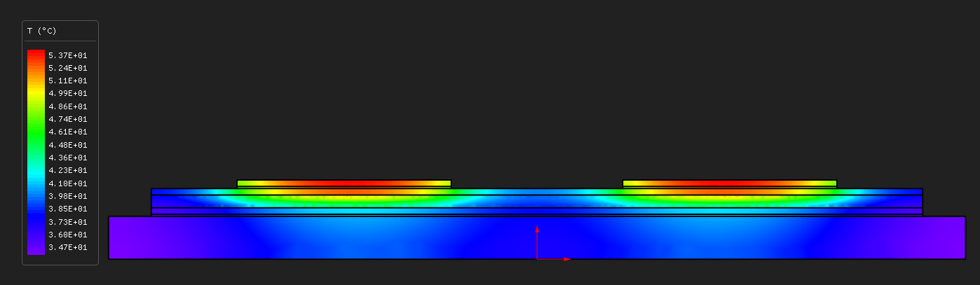
Check	Result	Tolerance
h·A·(T̄bottom − T∞) vs the 200 W dissipated	0.19 %	3 %
(convection Rth) − (fixed-temperature Rth) vs 1/(hA)	5.98 %	15 %
FEM junction rise vs the 1-D stack estimate Σt/(kA)	4.4 %	20 %

The second one is not expected to be zero: with a Dirichlet bottom the cooled face is isothermal and with a film it is not, and the ~6 % residual is the baseplate's own spreading responding to that difference. The third is not expected to be zero either, and that is the point — the 1-D estimate takes every layer at the die's footprint area, so the gap between it and the FEM is exactly the lateral spreading the DBC copper and the baseplate provide. The FEM answer is the lower one; a stack estimate that came out below the FEM would mean the estimate was wrong.

Stage 2 — the pulsed transient

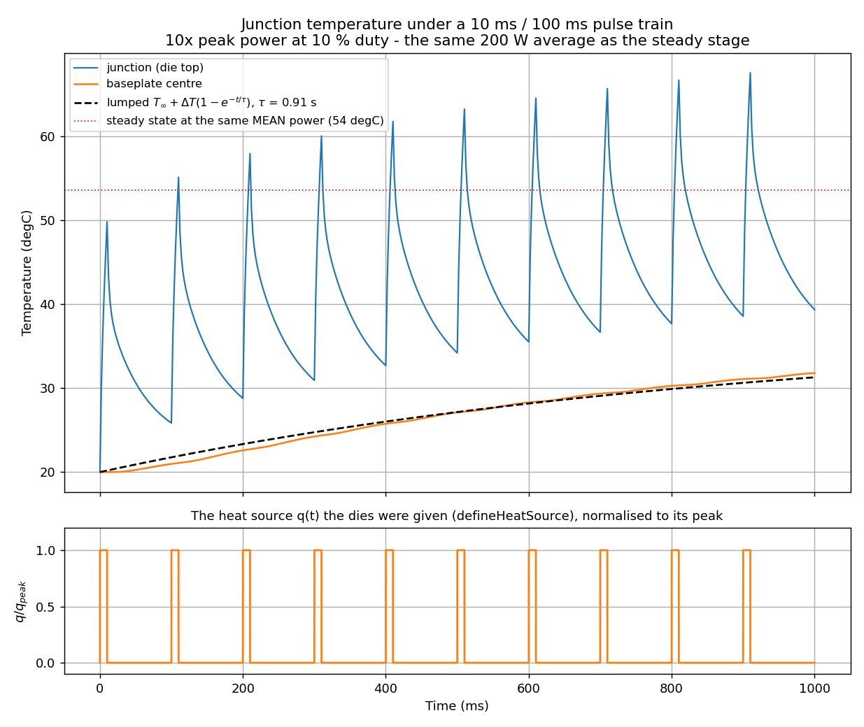
The same 200 W average, delivered as a 10 ms on / 100 ms period pulse train — 10 % duty, so ten times the peak power — for ten cycles from 20 °C. The engineering content is on the first pulse:

• Junction ripple is 29.0 K peak to peak, and the very first peak already reaches 50 °C — within 4 K of the final steady-state junction temperature, at a moment when the baseplate has not moved at all. A module sized on average power is sized wrong.
• The slow part — the baseplate — rises with a fitted time constant of 0.915 s toward the steady stage's own 17.0 K.

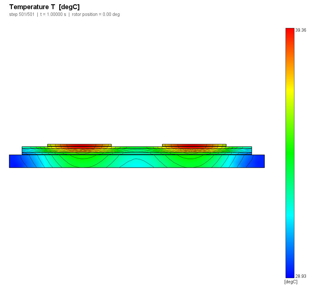
The lumped anchor is τ = CeffR: 0.863 s against 0.915 s fitted, 6.0 % apart. Ceff is not the module's bare mass, and the difference is worth the four lines it costs. A single pole matches a distributed system when it stores the same energy at the same reference temperature, and the stack above the baseplate sits much hotter than the baseplate does — the dies at twice its rise. Each region's heat capacity therefore enters weighted by how hot that region actually gets:

C_eff = sum_i  C_i * (T_i - T_inf) / (T_ref - T_inf)     from the STEADY solution

which gives 10.17 J/K against a bare mass of 8.87 J/K. Using the bare mass makes τ come out 18 % short, and the size of that error is precisely the heat the DBC stack is holding. The script reports both.

The transient runs on a mesh about half the size of the steady one, because it writes one full nodal record per step. What that costs is measured, not asserted: the steady state is re-solved on the coarse mesh before any transient number is believed, and its junction temperature lands 0.08 % of the junction rise away from the fine-mesh answer.

Stage 3 — one line of code, 8.9 K

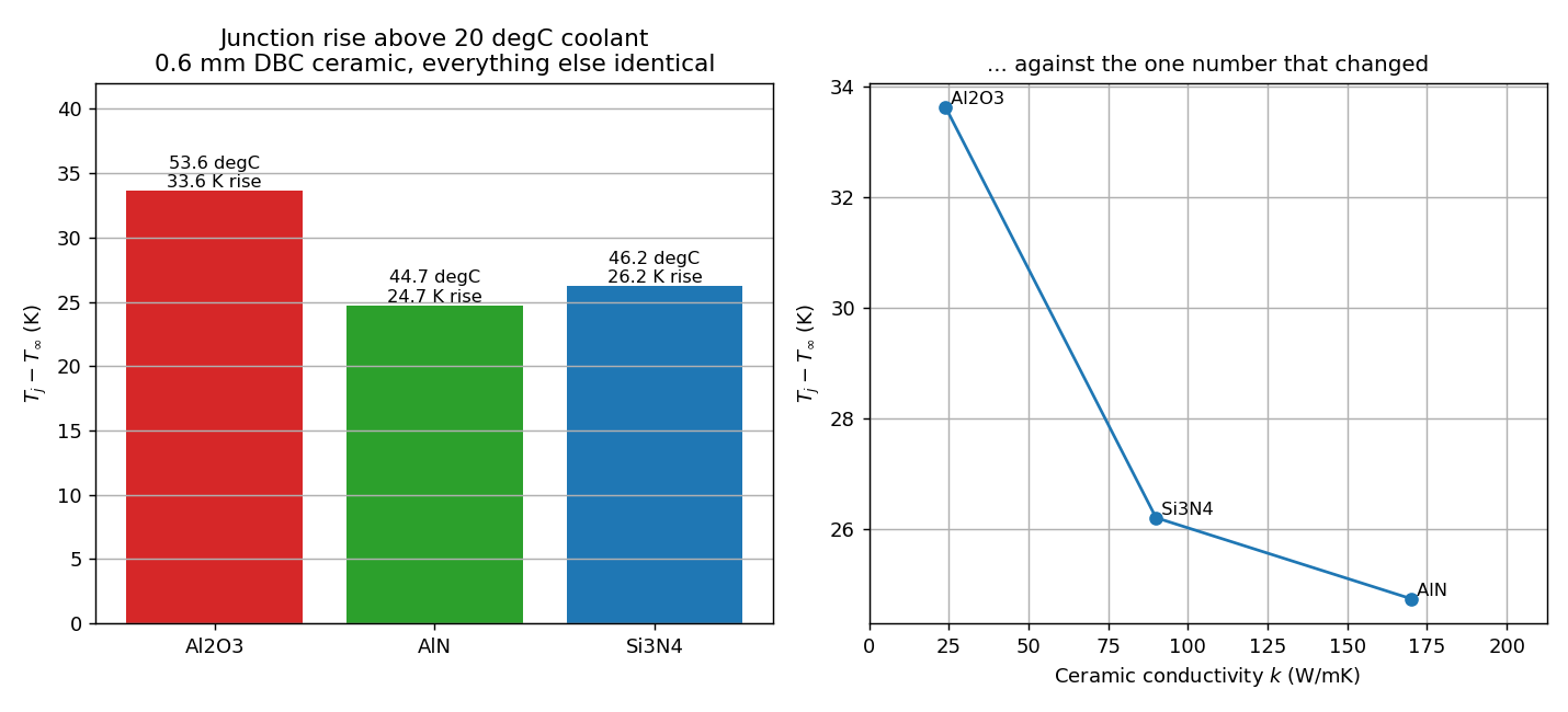
The DBC ceramic is swapped and nothing else moves — one property call.

Ceramic	k (W/mK)	Tj	Rise above coolant	Rth
Al2O3	24	53.6 °C	33.6 K	168.1 mK/W
Si3N4	90	46.2 °C	26.2 K	131.0 mK/W
AlN	170	44.7 °C	24.7 K	123.7 mK/W

AlN instead of alumina is worth 8.9 K of junction temperature — 26 % of the whole rise, for one line of code. The curve also shows where it stops paying: 24 → 90 W/mK buys 7.4 K, and 90 → 170 buys 1.5 more, because by then the ceramic is no longer the bottleneck.

Traps this example respects

• Enabling the thermal module comes first. Thermal boundary condition types 20/21/22 and every thermal region property are refused before it.
• Conductivity, density and specific heat are per region and have no useful default. A region left alone conducts like whatever the default is, silently, and a wrong conductivity produces a converged, plausible, wrong temperature. All nine regions here are given all three from one table — which is also what the heat-capacity sum and the probe grid read, three things that must not be allowed to disagree about what the stack is.
• A region with an assigned heat source ignores its constant q. The constant is still set, because a steady run reads it even when a table is present.
• The pulse table is interpolated linearly and held flat outside its range, so a square edge is a 0.05 mm-wide ramp. The edges are placed so that with backward Euler — which evaluates the source at the end of each step — the steps carrying the on-power span exactly 10 ms.
• Coarsening barely helps on this model. The mesh is set by the layer thicknesses — a 0.1 mm solder film needs two elements across it whatever the area constraint says — so quadrupling every area moves the node count from 5341 to 2495 and the answers not at all. On a stack of thin layers, mesh cost is a geometry decision.

Running it

python power_module_thermal.py                  # all three stages, ~35 s - 1.5 min
python power_module_thermal.py --stage steady
python power_module_thermal.py --stage transient
python power_module_thermal.py --stage material-sweep

The script rebuilds itself from nothing: delete everything but the script and one run brings the directory back.

Try this next

• Drop the film coefficient to an air heatsink's and watch the ceramic sweep flatten. Which layer is the bottleneck is a property of the whole stack, not of the ceramic.
• Change the duty cycle at fixed average power. The ripple is what the die actually sees, and it is the number that decides a lifetime.
• Move the dies closer together. The 8 mm spacing is what keeps their spreading fields from overlapping much; closing it is the cheapest way to make the module worse.

About these numbers

This is a demonstration module, not a datasheet. Every figure on this page came out of the run described here at the settings the script ships with. For accuracy against a stated reference and tolerance, the validation dossier is where that question belongs.