Single-phase transformer — a hand-built coil on a hand-built netlist

← Back to the examples

What you need to run it: the Python API (Automation) plus Core Pro, which is what the Crank-Nicolson time scheme needs. The script reports a missing entitlement rather than crashing, and deliberately does not fall back to Backward Euler — that would quietly build a different model than the one documented here.

What this one is for

This is the circuit-coupling workhorse of the set. Everything circuit-coupled in the shipped machine library is a squirrel cage built by the machine module; this is what you copy when you want to drive a hand-built coil from a hand-built netlist. If your model has a real source, a real load and windings you drew yourself, start here.

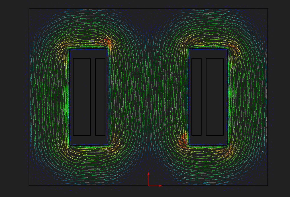
The device is a shell-type single-phase transformer: an E-I core with both windings on the centre limb, the flux splitting into the two outer limbs and closing through the yokes. 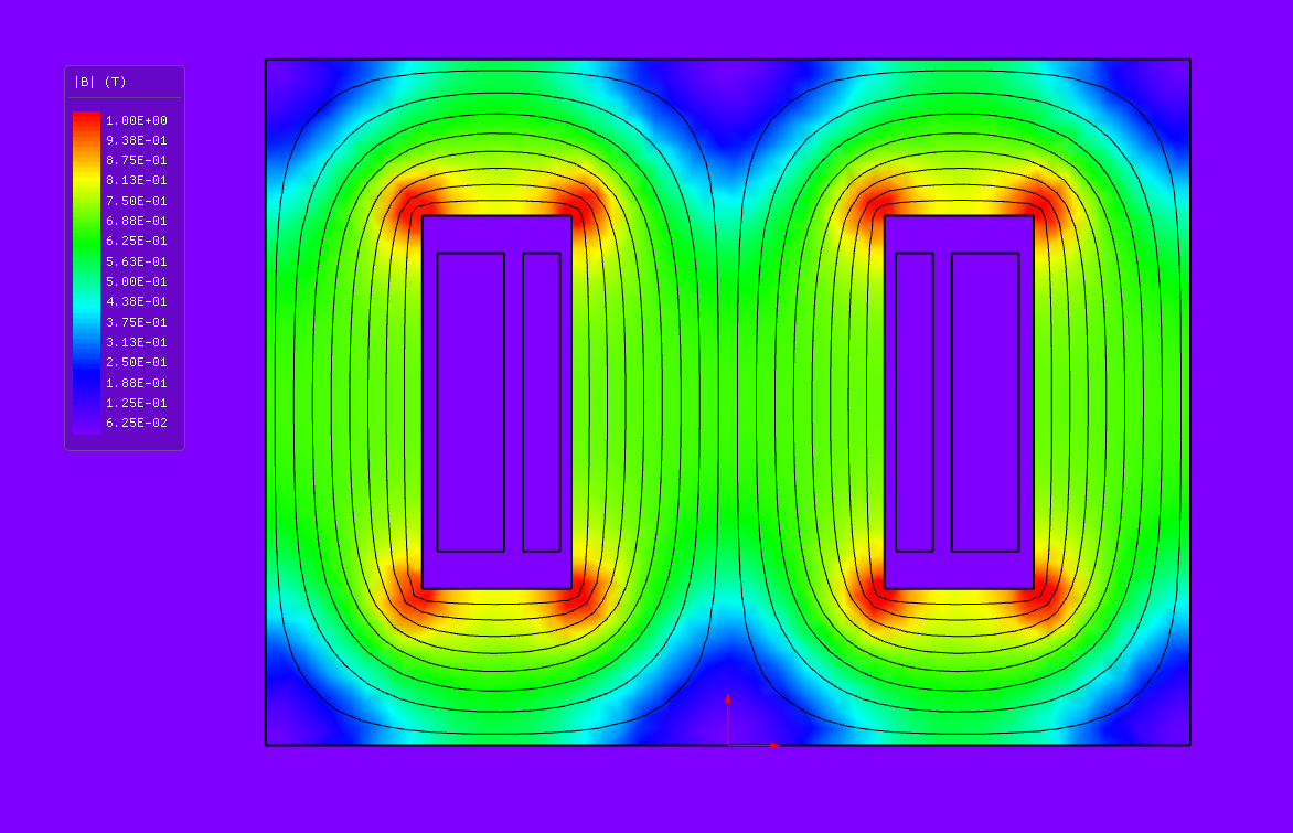Each winding is the standard 2D-FEM go/return pair — a left-window region carrying +Jz and a right-window region carrying −Jz, one loop around the same limb — with the primary inside, the secondary outside, and a real 5 mm air gap between them. That gap is the leakage path, and the field render shows what lives in it.

At a glance

Quantity	Value	Unit
Rating	2 kVA, 212.1 / 53.0 V rms, 50 Hz	—
Core	E-I shell type, centre limb 84 × 84, 84 mm stack, M-19 steel (BH)	mm
Primary / secondary turns	200 / 50 (a = 4)	—
Winding resistance (computed from geometry)	0.1456 / 0.0051	Ω
Load	1000	Ω
Primary current I1	0.0969	A rms
Primary terminal voltage V1	214.22	V rms
Secondary voltage / current	53.55 V / 53.03 mA	rms
Primary flux linkage peak	0.9547 (analytic V/ω = 0.9549)	Wb
Turns ratio V2/V1 vs N2/N1	0.01 (tolerance 3)	% off
Rated peak flux density	~0.68	T
Mesh	4312 nodes, P1	—
Run	3 periods × 100 steps, Crank-Nicolson, ~4 Newton iterations/step	—
Wall time, the 300-step solve	1:55 (1:06 with saturation off)	—

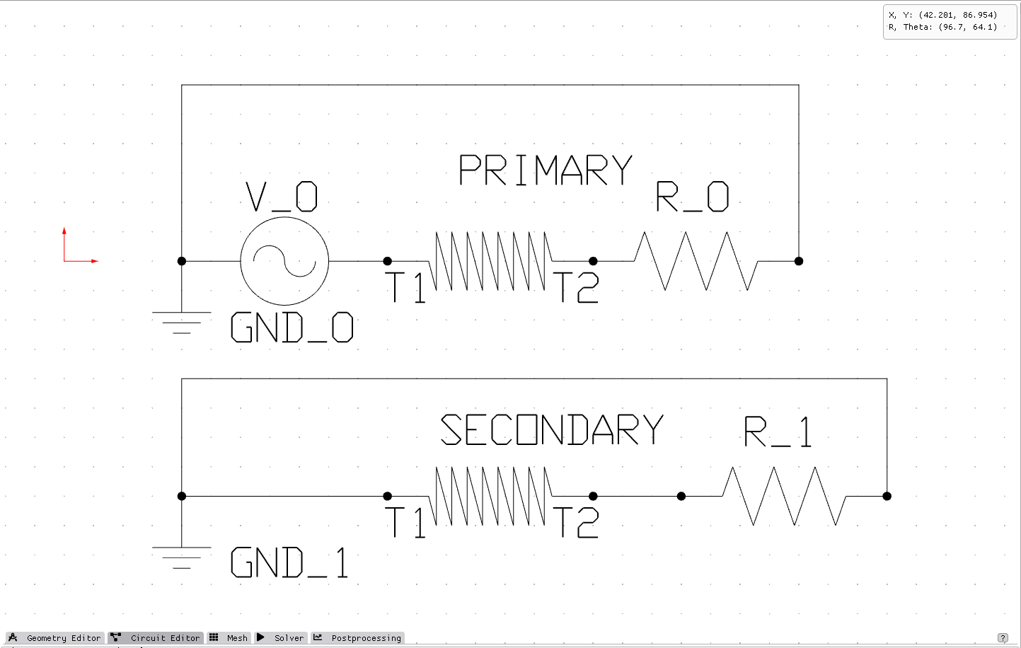
The netlist

V_0 (AC, 300 V peak, 50 Hz, phase 90 deg) -- CL:Primary -- R_0 (0.001 ohm) -- GND
GND -- CL:Secondary -- R_1 (1000 ohm) -- GND

Two independent loops, tied together only through the shared core flux. Nothing in the netlist connects them electrically, which matches a real two-winding transformer's galvanic isolation — and which is exactly why the turns-ratio check is the one that matters. The only way the secondary can develop a voltage at all is through the core, so recovering V2/V1 = N2/N1 to 0.01 % is the statement that the field-to-circuit coupling is doing its job.

R_0 is line and source resistance, not the winding's own. Both coils get a resistance computed automatically from their region geometry and conductivity; nothing in the script sets one by hand.

Two ordering rules are load-bearing and worth copying verbatim. Coil (CL) entries go on the circuit first, before the passives and the source — the solver warns when that is violated. And placement coordinates are not decoration: every pictogram's two terminals sit 70 units apart along its own axis, and the netlist is derived by matching wire endpoints to those terminals.

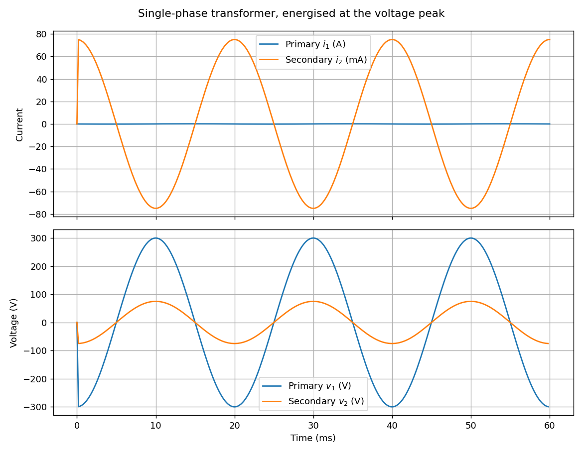
Energised at the voltage peak, on purpose

The source phase is 90°, so v(0) = +300 V: switch-on at the voltage peak. That is the benign case — the flux a settled sinusoid would already have at that instant is its own zero, which is exactly what the model starts from, so no offset is left behind and the run is in steady state almost immediately. The evidence is in the numbers: peak primary flux linkage comes out at 0.9547 Wb against the analytic V/ω = 0.9549 Wb.

Set the phase to 0° instead — a voltage zero-crossing, the worst case — and that peak roughly doubles, because the demanded flux λ(t) = (V/ω)(1 − cos ωt) never goes negative. That offset is real physics; it is the mechanism behind inrush. It decays only on the magnetising branch's own L/R time constant, which for this design is about 17 seconds — so three simulated periods would show it as an essentially constant DC bias on the current, not as something settling.

Saturation matters more than you would expect

This core's rated peak flux density is about 0.68 T, far below M-19's knee at 1.3–1.6 T. So “the core never saturates, the linear run should agree” sounds safe. It is not:

	Saturation on	Saturation off
Primary current I1	0.0969 A rms	0.2720 A rms (2.8×)
Secondary voltage V2	53.55 V rms	53.54 V rms
Secondary current I2	53.03 mA rms	53.02 mA rms
Flux linkage peak	0.9547 Wb	0.9548 Wb
Turns ratio error	0.01 %	0.03 %
Solve time, 300 steps	1:55	1:06

Two things are going on and both are worth knowing.

“Saturation off” does not mean “linear at the operating point”. With saturation disabled the solver does not fall back to the region's scalar μ — that would make the core air, and every number would be wrong by orders of magnitude. It seeds every element of a BH region with the curve's own initial permeability and leaves it there: μ_r = 2631 for M-19, the secant B/(μ0H) at that curve's first tabulated point.

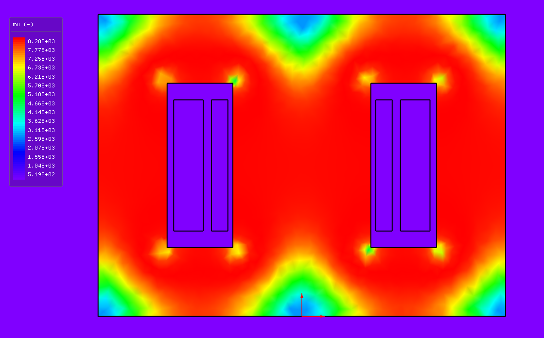
A soft magnetic material's permeability is not flat below the knee — it has a hump, and this core sits on top of it. M-19's μ_r climbs from 2631 at 0.05 T to a peak of 8284 at 0.70 T, then falls away into the knee. This transformer runs at 0.68 T. So the initial permeability the linear run uses is the curve's worst value, more than three times below the one that actually applies, and the magnetising current is correspondingly too big.

Everything except I1 is unchanged to 0.03 %, and that is not a coincidence: the flux is set by V/ω and the load branch by the turns ratio, and neither depends on μ at all. The magnetising current is the only reported quantity the material law really moves — which is exactly why an open-circuit test is how you measure a core in the first place.

A build bug worth recording

The first working version of this script never called defineAxialLength. Every other planar example in this set drives its coils directly, where the axial length only scales a reported quantity and its default is never load-bearing. Here it turned out to scale the coil's flux-linkage-to-circuit coupling itself: without it, every circuit-coupled coil in the model solved as a plain zero-impedance wire. The primary current tracked V(t)/R_0 exactly — a pure resistor response, jumping straight to V/R with no L/R rise at all — and the coil voltage read back a flat zero for the whole run.

It took three throwaway minimal models to isolate, and none of it was specific to a transformer or to AC. Call defineAxialLength on every planar model that has a circuit-coupled coil; the default silently zeroes the coupling rather than refusing to solve, so the failure mode is a plausible, converged, wrong run.

Core sizing: threading the saturation knee

M-19 turns sharply between 1.3 T and 1.6 T — a real knee, not a gentle curve. A good open-circuit demonstration wants the rated peak flux density comfortably below it (a small, near-sinusoidal magnetising current); a good inrush demonstration wants the transient's doubled flux excursion to land clearly above it. The two pull the core size in opposite directions, and the margin is narrow:

Centre limb × stack	Rated peak B (lumped estimate)	Open-circuit magnetising current	Inrush behaviour
58 × 70 mm	1.28 T	14.0 A rms (161 % of rated)	already saturated at rated flux — not a usable design
72 × 80 mm	0.90 T	4.04 A rms (46 %)	still visibly saturated at rated flux
80 × 80 mm	0.81 T	1.54 A rms (18 %)	steady current already non-sinusoidal
84 × 84 mm (shipped)	0.73 T	0.49 A rms (5.6 %)	clean sinusoidal OC current; the inrush peak flux sits right at the start of the knee
90 × 90 mm	0.64 T	0.21 A rms (2.4 %)	inrush flux stays under the knee — nothing to show

The table was measured at an earlier 230 V rating, so read the flux densities as proportional guidance rather than as this configuration's numbers. What it shows is that the lumped estimate B = V1/(4.44 f N1 A) is a poor predictor near the knee: the window's four inner corners are reentrant, and the field concentrates there the way it does at any sharp reentrant corner in a magnetic circuit. That is a real effect, not purely a meshing artefact, and it is why the 72 and 80 mm rows already look saturated at a “should be fine” lumped estimate. The shipped size was found empirically — that table is the search.

Running it

python transformer_1ph.py            # the full run, ~2.5 min
python transformer_1ph.py --coarse   # every mesh area x4, a fast first look
python transformer_1ph.py --no-solve # build + mesh + save, solve nothing

Try this next

• Set the source phase to 0° and watch the flux excursion double into the knee. That is the inrush regime, where saturation changes the shape of the current waveform and not just its amplitude.
• Short the secondary and the same model becomes a short-circuit test: the leakage gap between the windings stops being scenery and becomes the only thing setting the current.
• Turn saturation off and compare, with the table above in hand. It is the cheapest possible lesson in what a linearised core actually assumes.

Two API quirks this script works around

• Tolerance and iteration limit are only applied when saturation is on — they are the nonlinear Newton loop's settings, and with a linear core that loop never runs. The script lands them with one priming call and then overrides the option bits, so the stored model matches the reference exactly.
• The coil result series do not share one time axis. Current returns one more sample than voltage, which is undefined at t = 0. Every row is [time, value], so use each series' own time column — zipping a single shared axis onto them silently shifts one series by a time step, which is small enough to look right and wrong enough to matter in an RMS ratio.

About these numbers

This is a demonstration transformer, not a catalogue part. Every figure on this page came out of the run described here at the settings the script ships with. For accuracy against a stated reference and tolerance, the validation dossier is where that question belongs.