Tubular pull-in solenoid — force and inductance over the stroke

← Back to the examples

What you need to run it: the Python API (Automation) and nothing else — a static P1 run, planar or axisymmetric, is Core. The script checks up front and exits cleanly with a message rather than failing at the solver.

What this one is for

This is the axisymmetric primer of the set. Model x is the radius r (never negative), model y is the axial coordinate z, the axis carries a Neumann symmetry boundary, and the solver integrates over 2π — so there is no defineAxialLength anywhere in the script and every force below is the force on the whole ring of material, not a per-metre figure. If you are about to build a rotationally symmetric device, read this one before the coilgun, which is the same formulation with three more moving parts.

The device itself is the everyday one: a steel plunger pulled into a coil, with a shell that gives the flux somewhere to return. What the example is really about is the pair of numbers an actuator is designed on — F(x) and L(x) — and the fact that they are two views of the same solution and can be made to check each other.

At a glance

Quantity	Value	Unit
Plunger (moving)	Ø10 × 30, 1020 steel, nonlinear BH	mm
Shell	pole plate 14 mm dia × 6 thick, guide bore 5.25 mm, return wall to 14 mm dia	mm
Seat boss	3 mm dia × 1.5 tall cone, apex on the axis	mm
Drive coil	ID 12, OD 24, 40 long, N = 800	mm
Domain	r in [0, 60], z in [−40, 100], Dirichlet A = 0	mm
Stroke swept	0 (closed) to 20 (open), 11 positions	mm
Currents	0.5, 1.0, 2.0	A
Axial force, closed, at 1.0 A	−2.005	N
Force reverses sign at	9.6 (at 0.5 A)	mm
Coil inductance, closed / open, at 1.0 A	62.19 / 45.07	mH
Eggshell vs virtual work, at 2.0 A	12.1 worst case	%
Mesh	~2600–2700 nodes per solve, P1	—
Wall time, 33 static solves	40	s

The seat is a real mechanical stop

The pole's top face carries a small conical boss whose apex sits on the axis, and a flat-faced plunger approaches it and stops 0.3 mm short. That is not a numerical fudge to keep the mesh alive — it is what a real design does, so that the plunger contacts the pole at one point rather than face to face, which is what stops it sticking shut on remanence when the coil is de-energised. The gap it leaves is smallest on the axis and widens with radius, and that shape is the “seat” the device is named for.

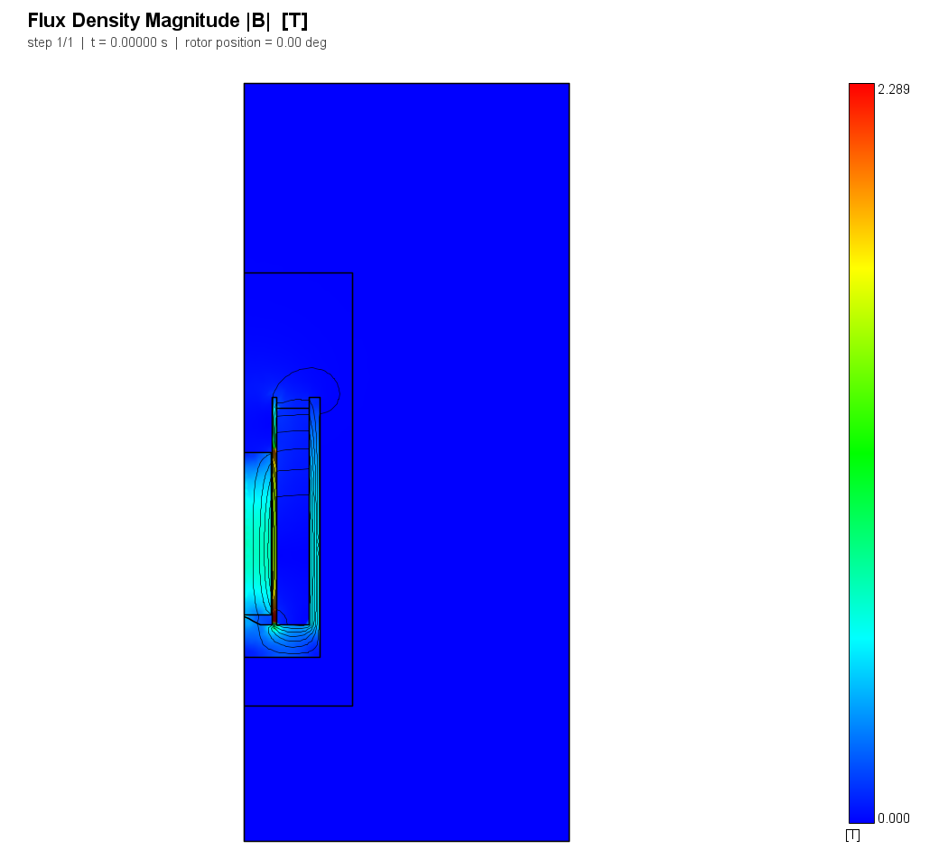
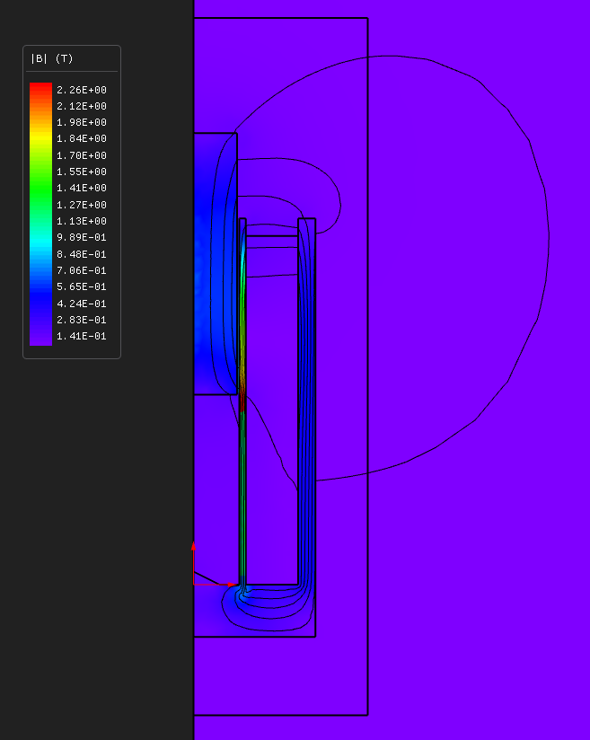
Closed, the seat boss is visibly past 2 T — it is the smallest cross-section in the loop and it saturates first. Open, the same current produces almost nothing across the seat, and the flux that remains is circulating in the return wall.

The stroke sweep

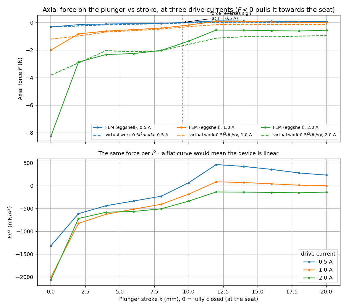
Eleven positions × three currents = 33 static solves, geometry rebuilt and remeshed at each point. Per point the script reads, immediately after that point's own solve, the eggshell axial force on the plunger and the coil's flux linkage.

The force reverses sign partway along the stroke, and that is real rather than an artefact — both the eggshell force and the virtual-work overlay agree on roughly where. Near the seat the coil pulls the plunger further in; far enough out, the balance shifts and it very weakly pushes the other way. The figure marks the crossing.

Underneath the force is F/I². If this device were magnetically linear that curve would be flat. It is not, which is the shortest possible statement of why the whole sweep is run at three currents instead of one and scaled.

Inductance, and the check it buys

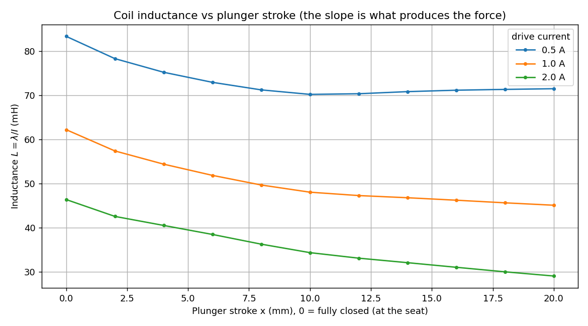
L(x) = λ/I falls smoothly and monotonically from 62.2 mH closed to 45.1 mH open, and its slope is what produces the force. The classical identity F = ½I²·dL/dx is therefore an independent route to the same number — a global circuit derivative against a local stress integral, on the same solutions.

They agree closely over part of the stroke, and the reason they do not agree everywhere is worth understanding before you copy the check into your own model. The return wall this device needs for a useful force is also a complete, low-reluctance magnetic loop that never touches the plunger — removing it drops the coil's inductance by roughly half. Wherever that stroke-independent loop's share of L(x) is comparable to the seat gap's, the derivative is being taken of a sum dominated by a term that carries none of the force. The identity is still exactly true in the continuum; it is numerically fragile there.

The consequence inverts the usual advice. The comparison is best at the highest drive current, not the lowest: the seat boss saturates locally, and saturation there makes the seat's own reluctance dominate the total instead of the fixed parasitic loop. So the check is gated at 2 A (12.1 % worst case) and reported without gating at 1.0 A and 0.5 A (18.5 % and 83.3 %). Points near the force's own zero crossing are excluded for the ordinary reason that comparing two numbers near zero is not a check.

Two wrong turns, kept on the record

Building the return path took two attempts, and both are the kind of thing that costs an afternoon:

• No return yoke at all. Plunger, shell and coil with the flux closing only through far-field air measures forces under a millinewton and an inductance that increases with stroke — backwards. With no local low-reluctance path the loop's reluctance is dominated by the huge external air path rather than by the seat gap, and the seat physics is drowned in leakage. The shipped model adds a return wall beside the coil.
• A missing shared edge. The coil's outer wall must be split at the coil's own top, not just where the guide tube ends further up, because its inside neighbour changes from coil to open air exactly there. Leaving that edge out let the mesher flood one region's material across the crack and produced a force spike that survived three levels of mesh refinement — convincing enough to be mistaken for physics. A “mesh-converged” spurious result is still spurious: convergence only proves the wrong mesh is being refined consistently.

Running it

python solenoid_actuator_axi.py                # the sweep, ~40 s
python solenoid_actuator_axi.py --coarse       # every mesh area x4, under 15 s
python solenoid_actuator_axi.py --currents 1.0 # one current only

Working axisymmetrically

The restrictions are worth knowing before you draw anything: geometry lives in x ≥ 0 only; rotary motion and the arc periodic and band boundary conditions (types 3/4/5/6) are rejected; skew is rejected; nodal B on the axis itself scatters by roughly ±10 %, so probes go slightly off-axis; and setProblemType must be called before meshing. The seat boss reaching r = 0 is a genuine axisymmetric point, and the mechanical 0.3 mm clearance is what keeps every swept position meshable.

Try this next

• Remove the return wall and watch both curves collapse. It is a two-line edit and it is the fastest demonstration of why the return path is the first thing an actuator design gets right.
• Flatten the seat. Replace the conical boss with a flat pole face and the closed-position force climbs sharply — and so does the residual holding force after the coil is switched off, which is the trade the boss exists to make.
• Push the current up. The saturation that makes the virtual-work check work at 2 A is also what flattens the force, so there is an optimum drive somewhere and this sweep is how you find it.

About these numbers

This is a demonstration actuator, not a catalogue part. Every figure on this page came out of the run described here at the settings the script ships with. For accuracy against a stated reference and tolerance, the validation dossier is where that question belongs.