Assumptions
This case study focuses on a 2D transient simulation of a Permanent Magnet Synchronous Motor (PMSM) using Nabla. The motor consists of a stator with three-phase windings and a rotor with embedded permanent magnets. To reduce the computational time only a 60-degree sector of the motor is modeled, leveraging the motor's geometric and electromagnetic symmetry. The simulation aims to analyze the magnetic field distribution, torque production, and back-EMF characteristics during operation.
Parameters
- 6-poles and 18-slots PMSM
- Axial length: 100 mm
- Stator outer diameter: 160 mm
- Permanent magnet parameters: (Br = 1.256 T, Hc = 1000 kA/m)
- Operating speed: 5000 RPM
- Frequency: 250 Hz
Geometry
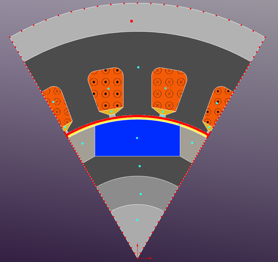
The 2D cross-sectional geometry (PMSM.dxf) of the motor is created using CAD software and imported into Nabla. The geometry includes the stator core, rotor core, and permanent magnets, rotor sleeve, shaft, etc.
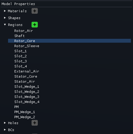
Regions
The geometry is divided into several regions representing different materials:
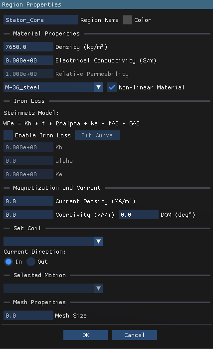
- Stator Core: Silicon Steel M-36
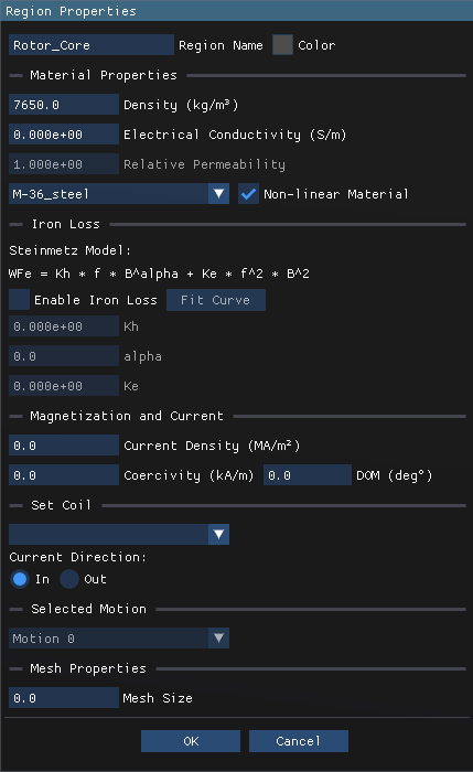
- Rotor Core: Silicon Steel M-36
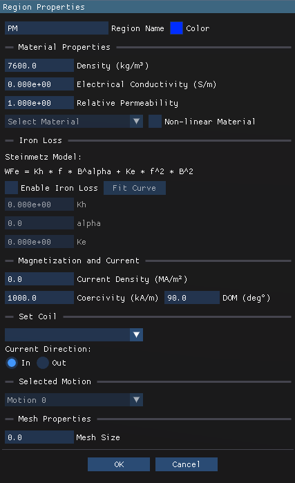
- Permanent Magnets: (Br = 1.256 T, Hc = 1000 kA/m)
- Air Gap: 0.5mm
- Rotor Sleeve: 1.0mm non-magnetic μ = 1
- Winding Regions: copper - stranded conductors (eddy-currents disabled)
- Shaft: non-magnetic μ = 1
Region Properties
The region properties are defined as follows:
Boundary Conditions
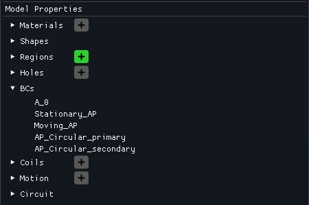
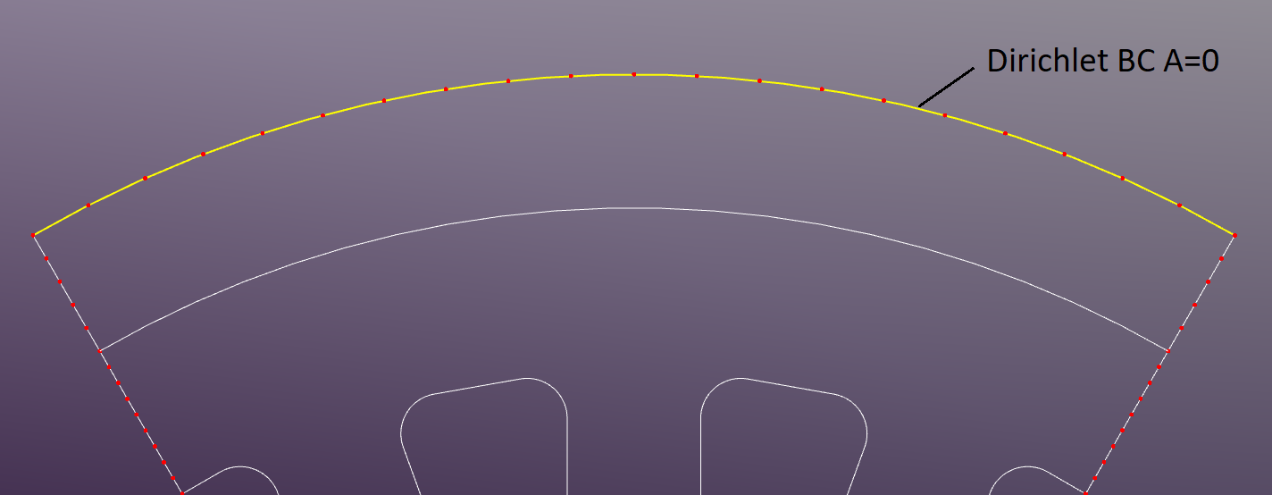
The outer boundary of the model is set as a Dirichlet boundary condition with a fixed magnetic potential of zero.
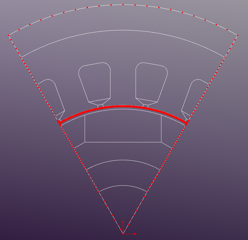
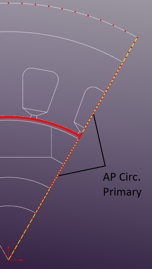
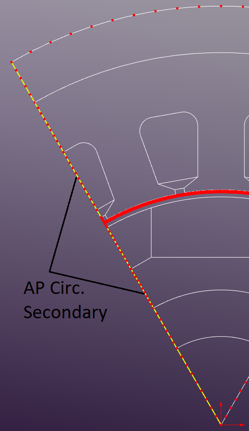
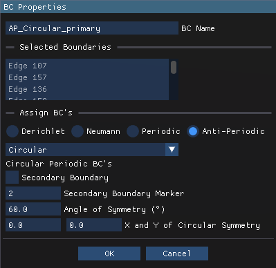
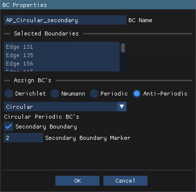
"Anti-Periodic Circular" BCs are applied to the left and right edges of the 60-degree sector to simulate the motor's rotational symmetry. AP_Circular_Primary includes the edges on the right side of the sector, while AP_Circular_Secondary includes the edges on the left side. 60-degree angle of symmetry implies that the primary side is rotated 60 degrees relative to the secondary side and matched accordingly. It's also important to note that the "secondary boundary marker" must be set to the same value in the primary and secondary AP BCs (see images below).
Coils
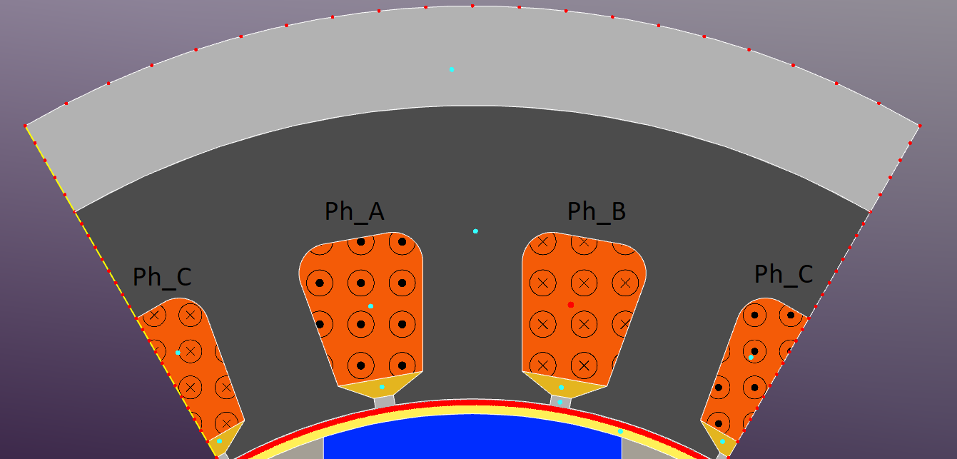
The Motor Coils are defined in the Model Properties section. Each coil is assigned to a specific region representing the winding area and given electrical parameters such as current amplitude and phase angle.
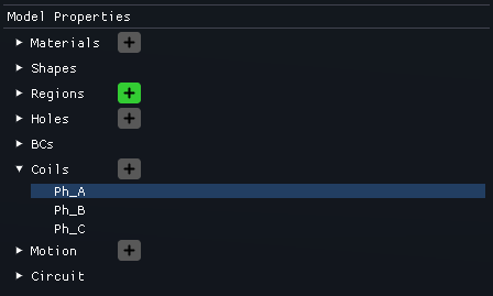
There are two ways to assign coils to regions: in the Region Properties in the corresponding "Set Coil" section or interactively in the main graphical window by selecting the desired region and assigning the coil from the dropdown menu. The coils current direction (highlighted with the corresponding templates) should be set according to the motor's winding configuration (e.g., ABC phase sequence).
The Coil properties are defined as follows:
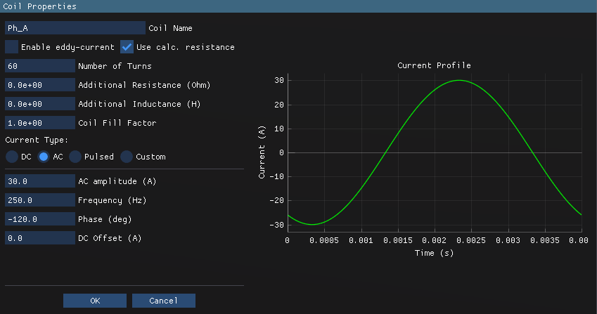
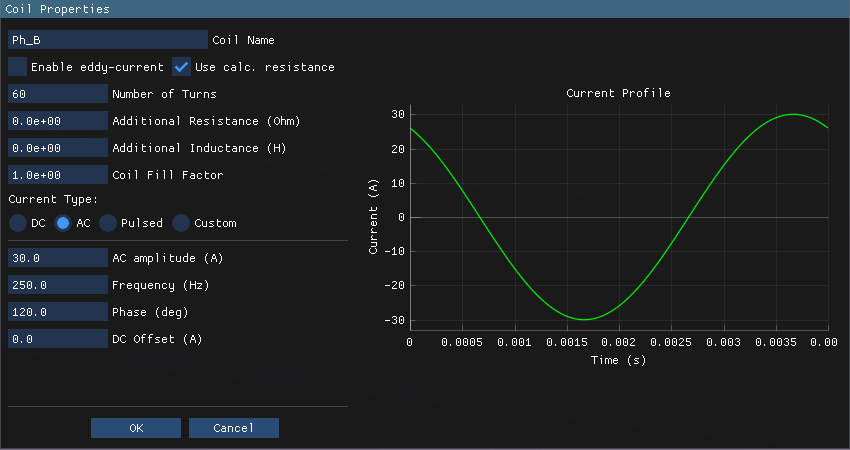
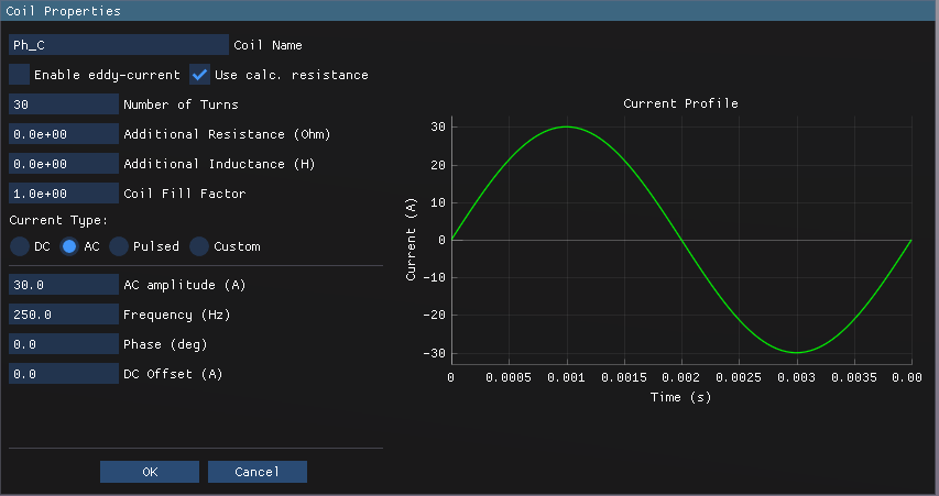
We're running the simulation in current-driven mode in this case study when the coil currents are specified directly. The phase currents are defined in a such way that Iq = 10 A and Id = 0 A. It should be noted that thecoil of Ph_C is splitted into two regions. Thereby both regions should have the same coil assigned to them but with opposite current directions and half number of turns.
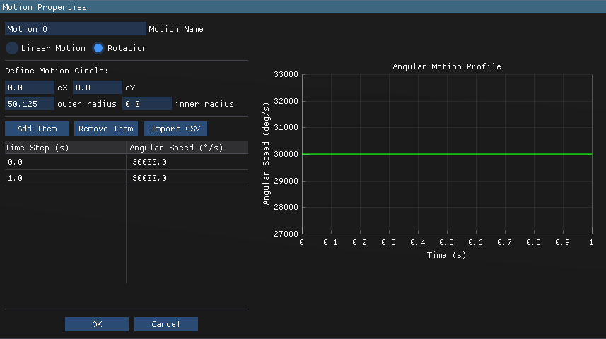
Motion
The motion region is defined as shown below: the rotor is set to rotate at a constant speed of 5000 RPM (250 Hz electrical frequency).
Meshing
The default mesh settings are used with a maximum element size of 1mm2
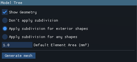
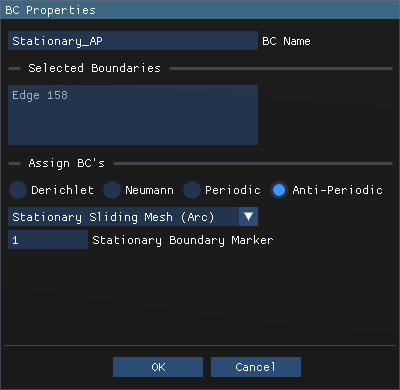
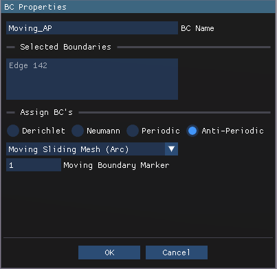
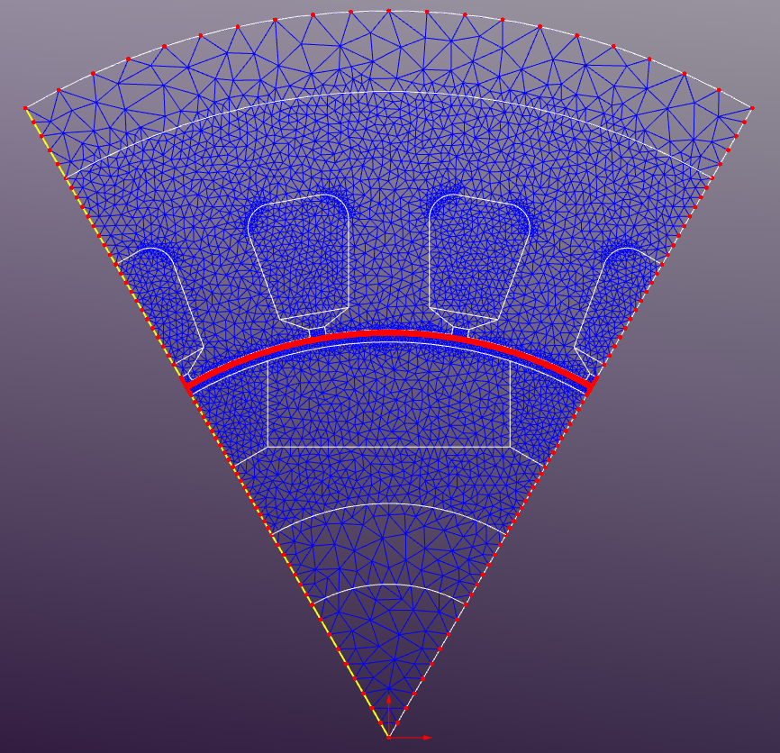
If the mesh size set to 0 in the Region Properties then the default mesh size will be applied to that region. The generated mesh consists of approximately 8910 triangular elements, with finer mesh density in the air gap and winding regions to capture the high field gradients accurately. An additional subdivision is applied to the edges with the boundary conditions to improve the solution accuracy near the boundaries. This is especially important for the sliding band edges where the number of elements should be the same on both sides to ensure proper field continuity during rotation. It is also recommended to subdivide the edges on the anti-periodic boundaries to get the same number of elements on both sides and enhance the solution accuracy. "Apply subdivision for exterior shapes" option should be selected in the Mesh Properties to enable this feature.
Results
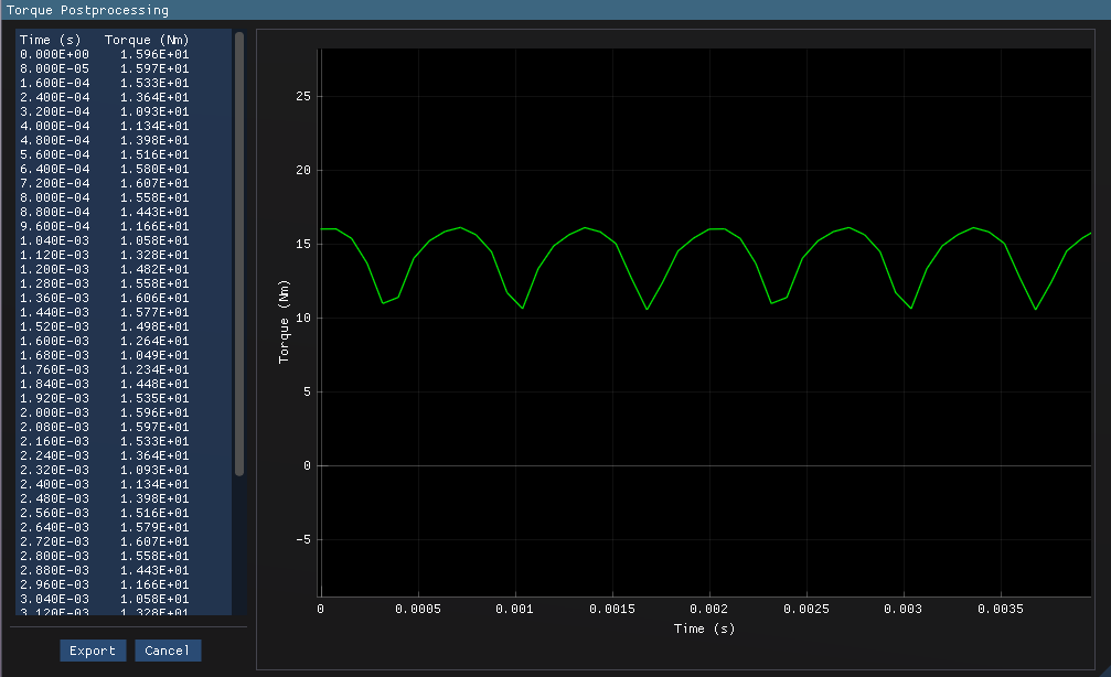
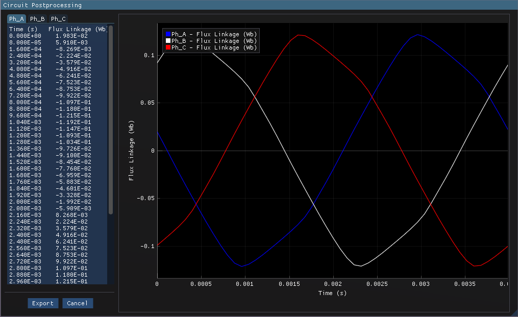
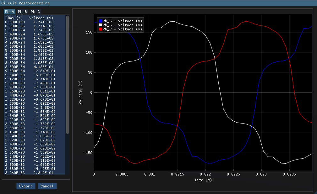
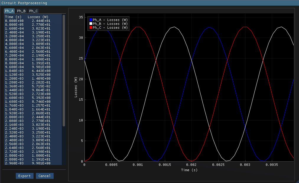
The simulation is run for a total time of 0.04 seconds with a time step of 8e-5 seconds, capturing one full electrical cycle at 250 Hz. The results include magnetic flux density distribution, torque production, flux linkage, phase voltage, back-EMF waveforms, instantaneous Joule loss in each slot. The torque produced by a single 60-degree sector is shown below. The total motor torque can be obtained by multiplying this value by 6.
An animation of the magnetic flux density distribution during motor operation is shown below.
Additional post-processing can be performed to extract more insights from the simulation data
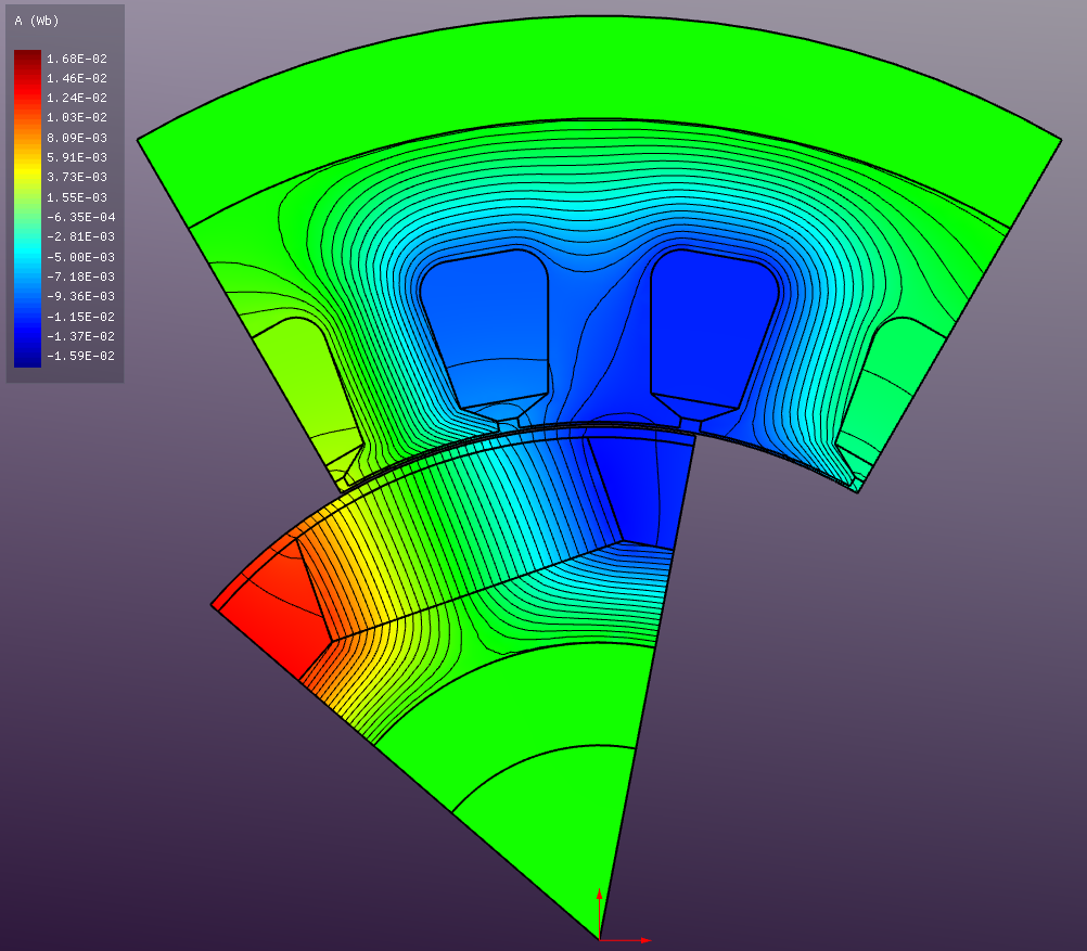
Vector Magnetic Potential (A)
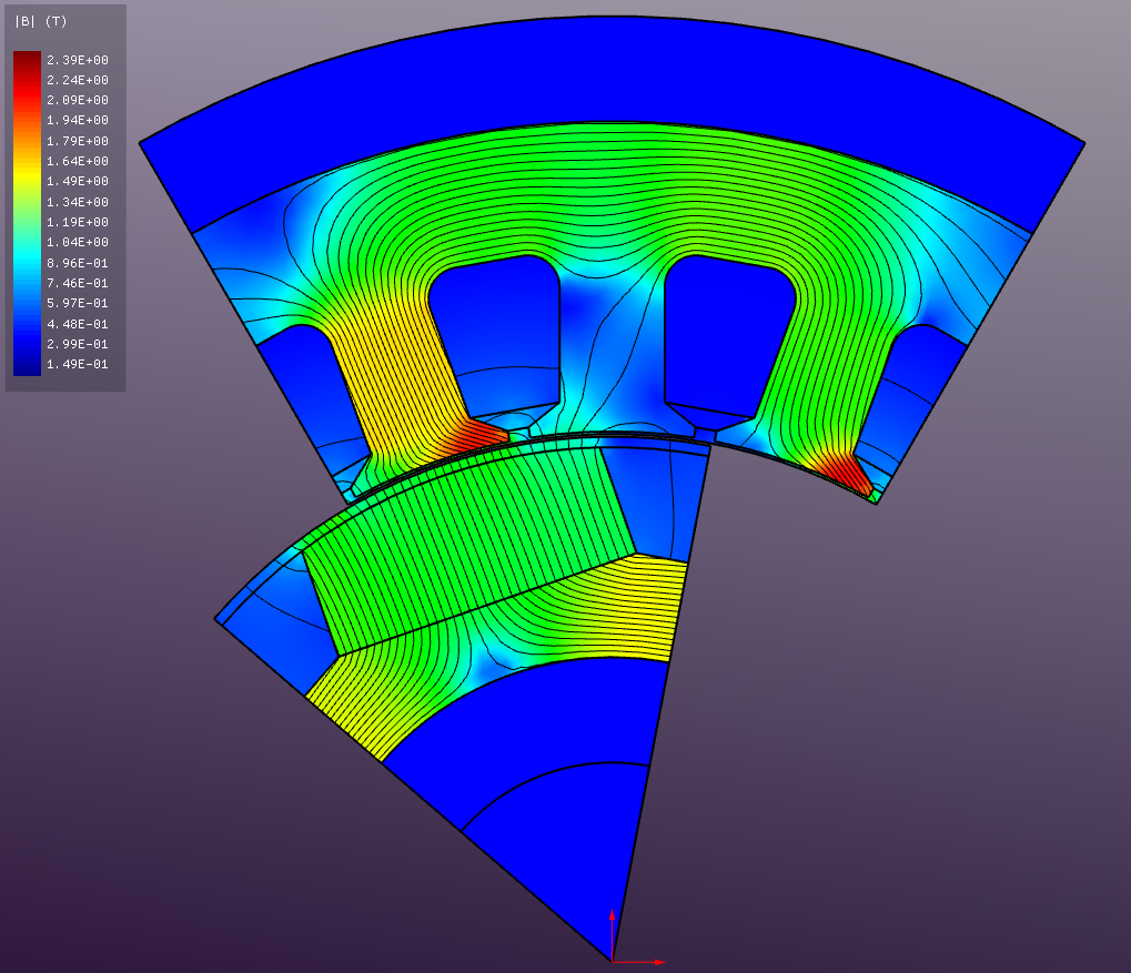
Absolute Magnetic Flux Density (B)
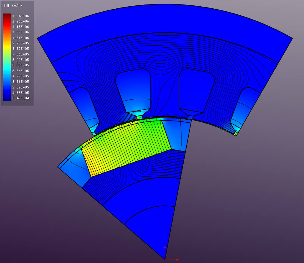
Absolute Magnetic Field Strength (H)
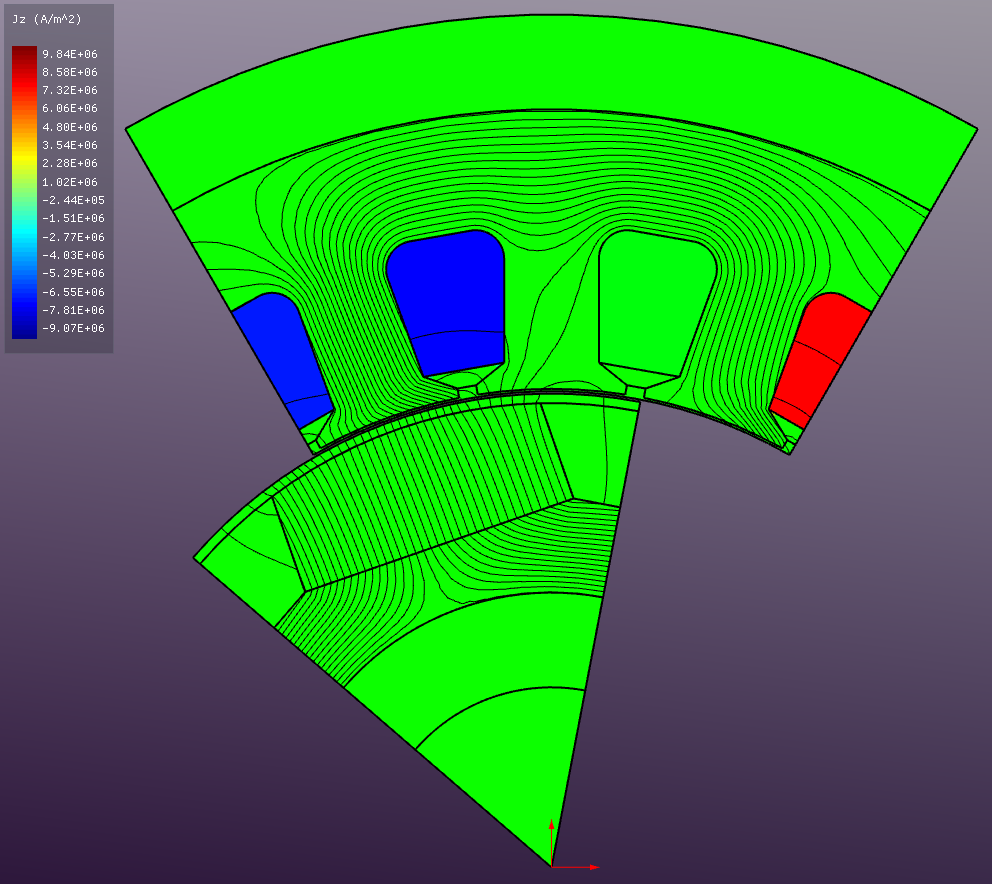
Current Density (J)
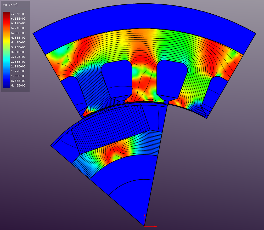
Relative Permeability (μ)
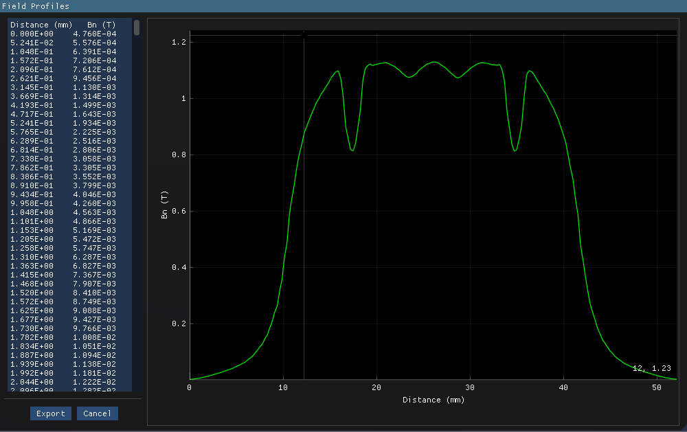
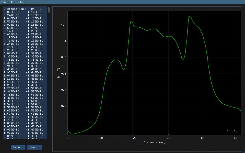
You can also extract the field distribution data along the specified path (or existing edges) within the model for further analysis. Here below is an example of the normal component of the magnetic flux density (Bnormal) in the air gap along a circular path at the rotor surface given for both no-load and loaded conditions.