Introduction
Nabla is a powerful finite element method solver designed specifically for
electromagnetic field analysis in low frequency domain. It provides researchers and engineers with the tools
to solve complex electromagnetic problems with high accuracy and efficiency.
Nabla is suitable for a wide range of applications including: machine design, transformer analysis, inductor modeling, etc.
Installation
View Installation Guide
Quick Start Guide
Step 1: Create Geometry
- Import CAD geometry or draw using built-in tools
- Define regions
- Assign material properties
Step 2: Set Boundary Conditions
- Identify boundary edges
- Apply appropriate boundary conditions
- Define excitation sources
Step 3: Generate Mesh
- Set mesh refinement parameters
- Generate the mesh
- Verify mesh quality
Step 4: Solve and Analyze
- Configure solver parameters
- Run the solver
- Visualize and analyze results
- Export data for further processing
Maxwell's Equations
Nabla solves various forms of Maxwell's equations depending on the problem type:
2D Magnetostatics
The magnetic field is computed using the vector potential A:
∇ × (ν∇ × A) = J
where ν = 1/μ is the reluctivity and J is the current density.
2D Time-Domain with Eddy-Currents
For transient problems including eddy-currents:
∇ × (ν∇ × A) + σ∂A/∂t = J
Geometry
Model geometry can be created using the built-in drawing tools or imported from standard CAD format: dxf
In-build tools allow creating basic shapes (lines, circles, rectangles) and combining them into complex geometries.
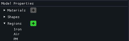
Regions
Material regions should be assigned to different parts of the geometry in the "Model Properties" pannel.
Each region can have different material properties such as permeability, conductivity, etc.
You can interractively select and assign regions in the graphics window. Regions are highlighted with distinct colors and a marker for easy identification.
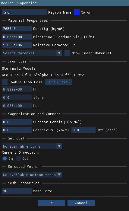
Region Properties
After defining regions in your geometry, you need to assign material properties to each region.
Nonlinear Materials
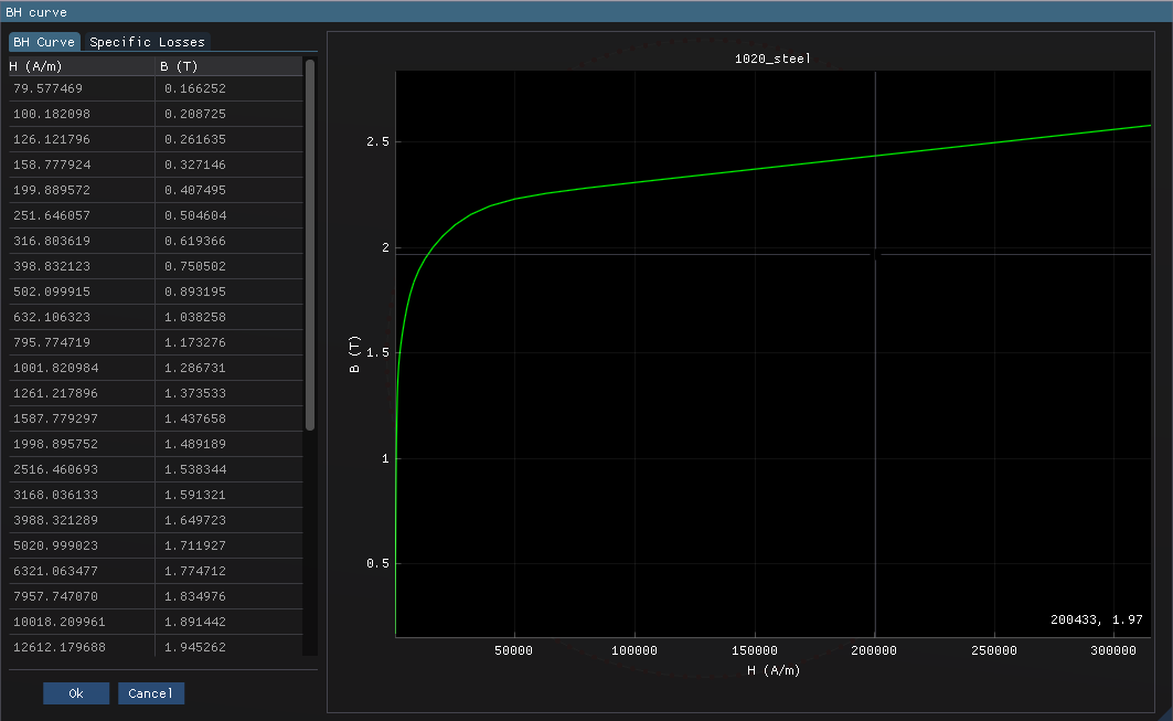
Nabla supports nonlinear magnetic materials by allowing users to define BH curves for regions.
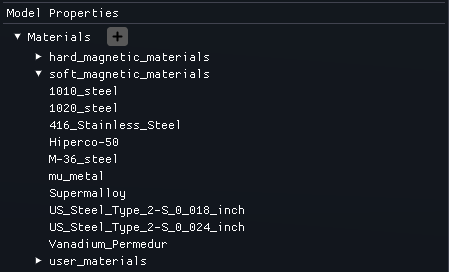
Materials section in the Model Properties pannel provides options to create user-defined nonlinear materials or select from a library of common materials.
BH curves can be input as tabulated data points or selected from predefined curves for standard materials like silicon steel, ferrites, etc.
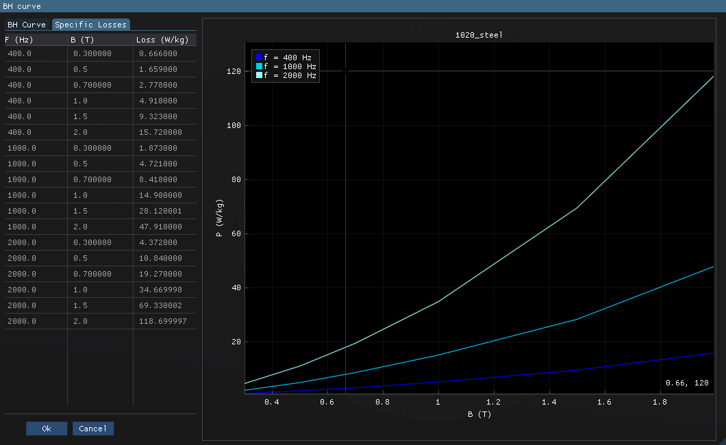
Nabla can compute Eddy-Current and Hysteresis (Iron) losses based on the defined specific loss curves.
The data should be defined as specific loss (W/kg) vs. peak flux density (B in Tesla) at different frequencies.
Nabla uses Steinmenz model for calculating Iron losses:
Piron = khfBα + kef2B2
Alternatively, users can provide Steinmenz coefficients kh, α, ke directly in the Region Properties Section of "Fit Curve" of selected material.
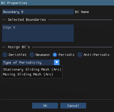
Boundary Conditions
Boundary conditions are applied to the edges of the geometry to define how the electromagnetic fields behave at the boundaries.
Select edges (use Ctrl+Click for multiple selection) in the graphics window and then "right-click" to open "Assign BC's" context menu for applying boundary conditions.
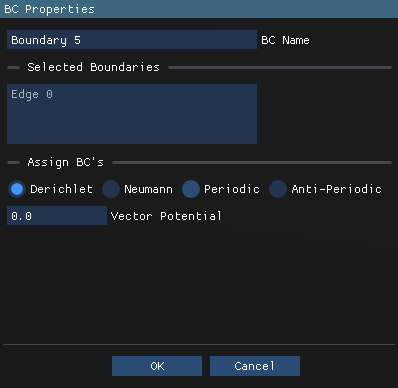
There are several types of boundary conditions available:
- Dirichlet - fixed potential
- Neumann - specified flux
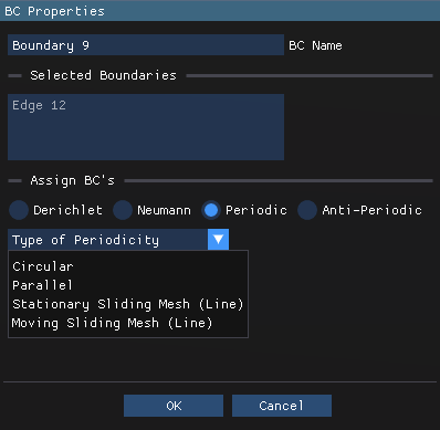
- Periodic
- Anti-Periodic
Periodic and Anti-Periodic boundary conditions are used to model repeating structures by linking pairs of edges.
For the linear edges the Periodic and Anti-Periodic BCs are applied as:
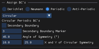
For arc and circle edges the Periodic and Anti-Periodic BCs are applied as:
Circular BCs can be used to model rotational symmetry by linking edges around a center point.
An angle of symmetry as well as a center point must be specified for the primary edge.
For the primary edge a "secondary boundary marker" (an unique integer identifier) must be specified to identify the linked edge.
For the secondary edge the "secondary boundary" checkbox must be selected and the same "secondary boundary marker" value must be provided.
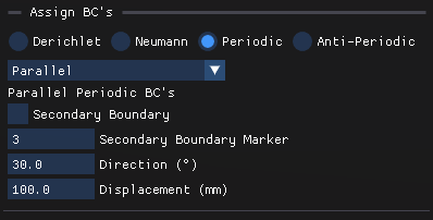
Parallel BCs are used to model symmetry along a line.
Similar to Circular BCs, a "secondary boundary marker" must be specified to link the primary and secondary edges.
The direction of the symmetry line and the distance from the primary edge to the secondary edge must also be provided.
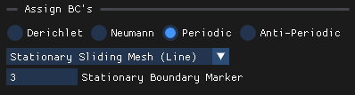
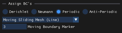
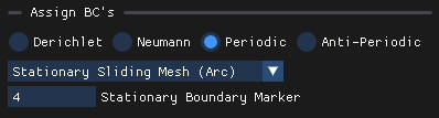
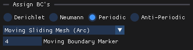
The special type of BCs: Stationary and Moving sliding mesh are used to model motion (linear or rotational) between two parts of the geometry.
This approach allows simulating relative motion without remeshing the entire geometry that saves computational resources.
Additional "sliding band elements" are created automatically in the region between the stationary and moving parts to ensure proper field continuity.
Excitation
Excitation sources such as current-carrying conductors or coils can be defined to drive the electromagnetic fields in the model.
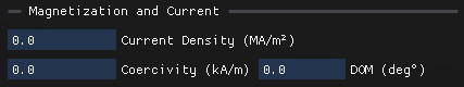
The excitation source can be assigned to in "Magnetization and Current" section of the Region Properties pannel:
Current density (MA/m²) for conductors or Coercive force (kA/m) & Direction of Magnetization for permanent magnets.
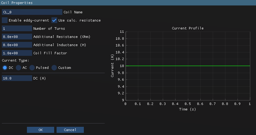
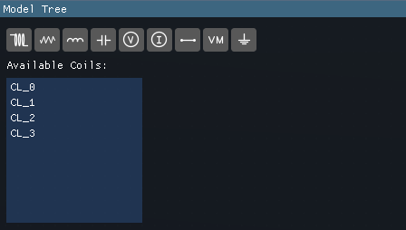
Another way to define excitation source is via Coil definition in the Model Properties pannel.
Then in the Coil Properties section, you can define coil parameters such as number of turns, current type, and additional coil properties.
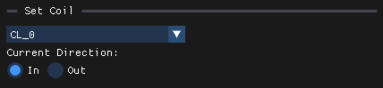
Then in the Region Properties pannel, you can assign the defined coil to a specific region by selecting the coil from the "Set Coil" section.
Alternatively, you can also assign coil to region via "right-click" context menu in the graphics window after selecting the region.
Meshing
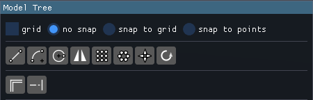
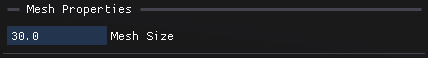
Mesh size can be specified for each region in the "Mesh Propertioes" section of the Region Properties pannel.
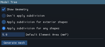
The default element size is defined in the Model Tree pannel.
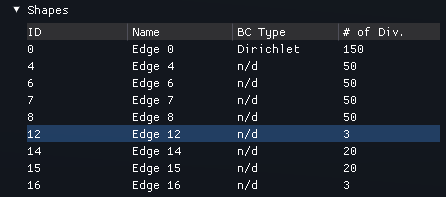
Nabla allows precisely controlling mesh density by specifying subdivisions for individual edges and then selecting the meshing method in the Model Tree pannel.
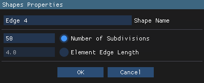
You can select edges in the Geometry Editor and then "right-click" to open the "Shape Properties" context menu for specifying the number of subdivisions or element edge length for the selected edges.
Alternatively, you can "Double-Click" on an edge in the Shapes list of the Model Properties pannel to open the Shape Properties dialog.
Circuit Editor
The Circuit Editor allows you to create and manage circuit components and connections within your model.
The Circuit Editor can be accessed from the Model Tree pannel by clicking on the "Circuit Editor" tab at the bottom of the main window.
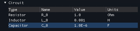
The following circuit components are available:
- Coil (if defined in the model)
- Resistor
- Inductor
- Capacitor
- Voltage Source
- Current Source
- Voltmeter
- Wire
- Ground
The Circuit EElements can be added to the circuit workspace by dragging and dropping them from the component list on the left side of the Circuit Editor.
Once added, you can connect the components by clicking on the terminals and dragging to create wires. You can orient the components using "Ctrl+R" keys.
Double-clicking on a component opens its properties dialog where you can set parameters such as resistance, inductance, capacitance, voltage, and current values.
You can also use "Circuit" section in the Model Properties pannel to define and manage circuit components.
Each circuit must have a ground component to establish a reference point for voltages in the circuit.
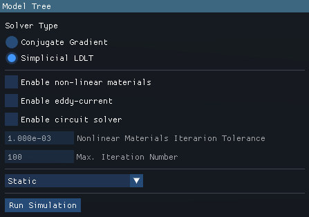
Solver Parameters
Solver parameters such as convergence criteria, maximum iterations, and solver type can be configured in the Model Tree pannel.
There are two solver types available in Nabla: Conjugate Gradient (CG) and Simplicial LDLT.
Conjugate Gradient is suitable for large sparse systems, while Simplicial LDLT is preferred for smaller dense systems.
Static or Transient analysis can be selected based on the problem requirements.
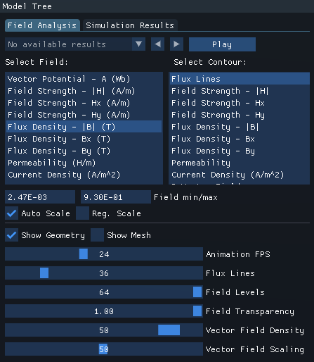
Postprocessing
Nabla provides various postprocessing tools to visualize and analyze the results via "Field Analysis" tab in the Model Tree pannel.
You can view field distributions, flux lines, and other relevant quantities directly in the graphics window.
Animation is supported for transient simulations to observe how fields evolve over time.
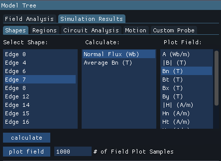
The "Simulation Results" section in the Model Tree pannel allows you more detailed analysis of the results:
- Field extraction along specified paths or edges
- Integral calculations such as Normal Flux, Joule Losses or Iron Losses
- Extract circuit parameters and export data for further analysis
- Extract torque for rotating machinery simulations
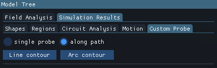
You can also specify custom paths in the graphics window via line or arc contours for extracting field data.
Shortcuts
Nabla provides several keyboard shortcuts to enhance productivity while working with the software:
- Ctrl+Left Click - multiple edge or region selection
- F2 - Rename selected item
- Ctrl+R - Rotate selected component (in Circuit Editor)
- Ctrl+I - Invert selected edges (in Geometry Editor)
- Ctrl+S - Save current model
- Ctrl+O - Open existing model
- Ctrl+N - Create new model
- Ctrl+Shift+S - Save As (the model will be saved in the current working directory)
- Delete - Delete selected item(s)
File Formats
Nabla model comprises and supports several file formats that store different aspects of the simulation setup:
- *.ujsn - unified JSON format for storing model data
- *.mfs - model for solver: an input file for solver
- *.poly - geometry data file: an input for
- *.dxf - CAD geometry file (if imported): a standard CAD format supported by many CAD software
triangle
mesh generator:
- *_solution.bin - binary file containing simulation results
- a bunch of files generated by
triangle
mesh generator:
API Reference
Coming soon...
Core Functions