V01 — Coaxial cable, long solenoid and current loop

← Back to the validation dossier

Tier A (analytic) - priority P0 Reference frozen on 2026-08-08. Nabla 0.1.0, solver licence mode enforcing, run in 23.6 s.

1. Problem

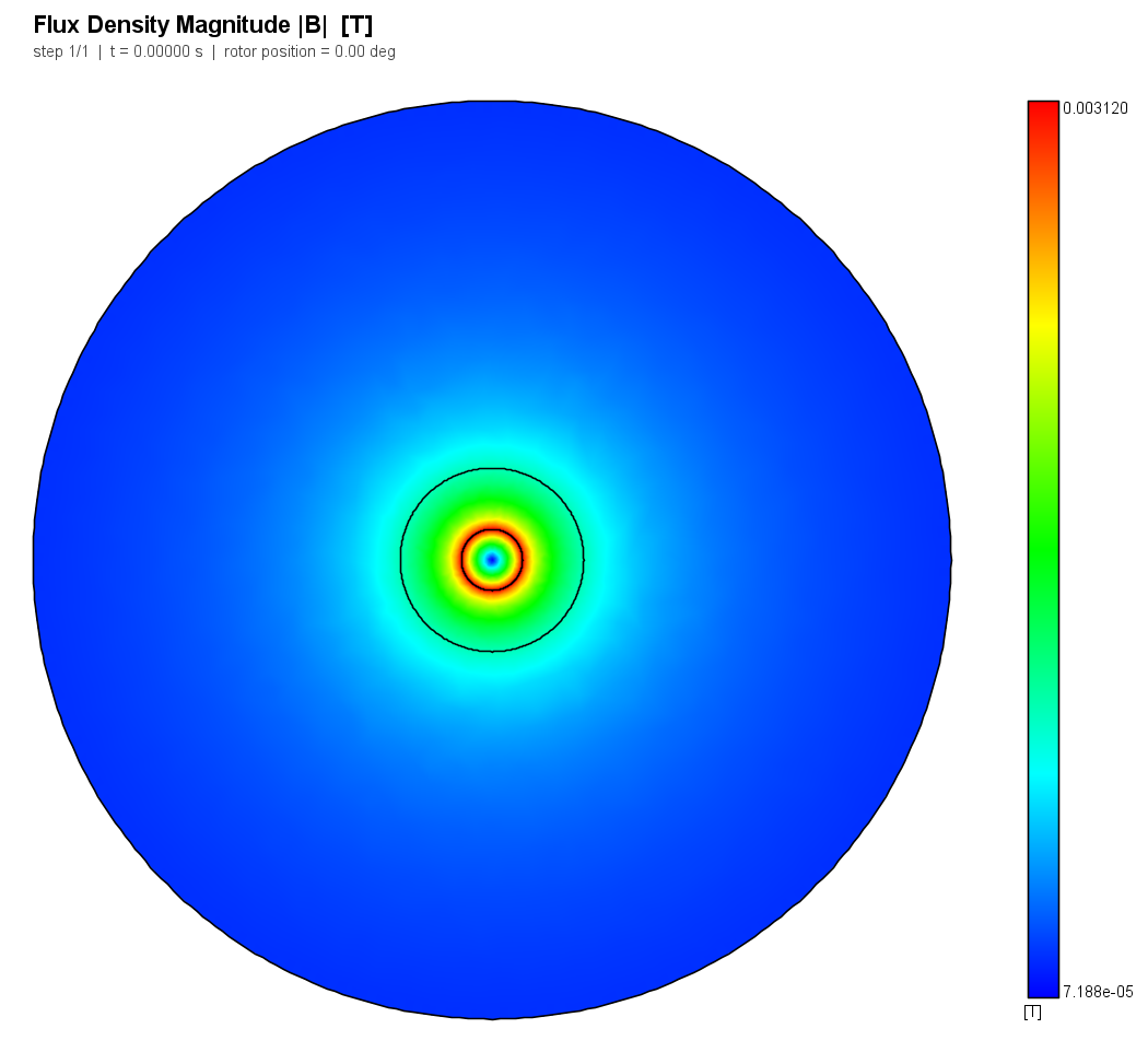
Three closed-form magnetostatic problems, chosen so that both 2D formulations and both element orders are exercised against answers nobody can argue with.

Sub-model	Formulation	Order	Geometry	Excitation
coax	Planar 2D	P1	round conductor r < 5 mm, dielectric to 15 mm, air to 75 mm	uniform J = 1 MA/m2 (78.54 A)
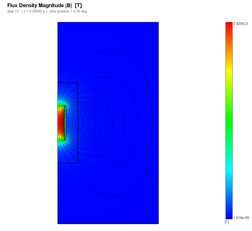
solenoid_p2	Axisymmetric 2D	P2	winding 20..25 mm radial, 100 mm long	500 A-turns
solenoid_p1	Axisymmetric 2D	P1	identical	identical
loop	Axisymmetric 2D	P2	ring of 10 x 10 mm section at 50 mm mean radius	1000 A-turns

The coax model carries an axial length of 1000 mm so that region field energies come out per metre directly. The axisymmetric models put a Dirichlet A = 0 boundary at ten times the coil radius and leave the symmetry axis natural (Neumann); the solver integrates over 2*pi, so no axial length applies.

2. Reference

All closed form, evaluated by harness/analytic.py at run time and compared against the values frozen in expected.json; a disagreement between the two is reported as DRIFT and fails the case.

• Round conductor. Ampere's law: B = mu0*I*r/(2*pi*a^2) inside, mu0*I/(2*pi*r) outside. Internal inductance mu0/(8*pi) H/m - independent of the conductor radius, and recoverable only from the energy stored inside the conductor. External inductance between two radii, mu0/(2*pi)*ln(r2/r1) H/m.
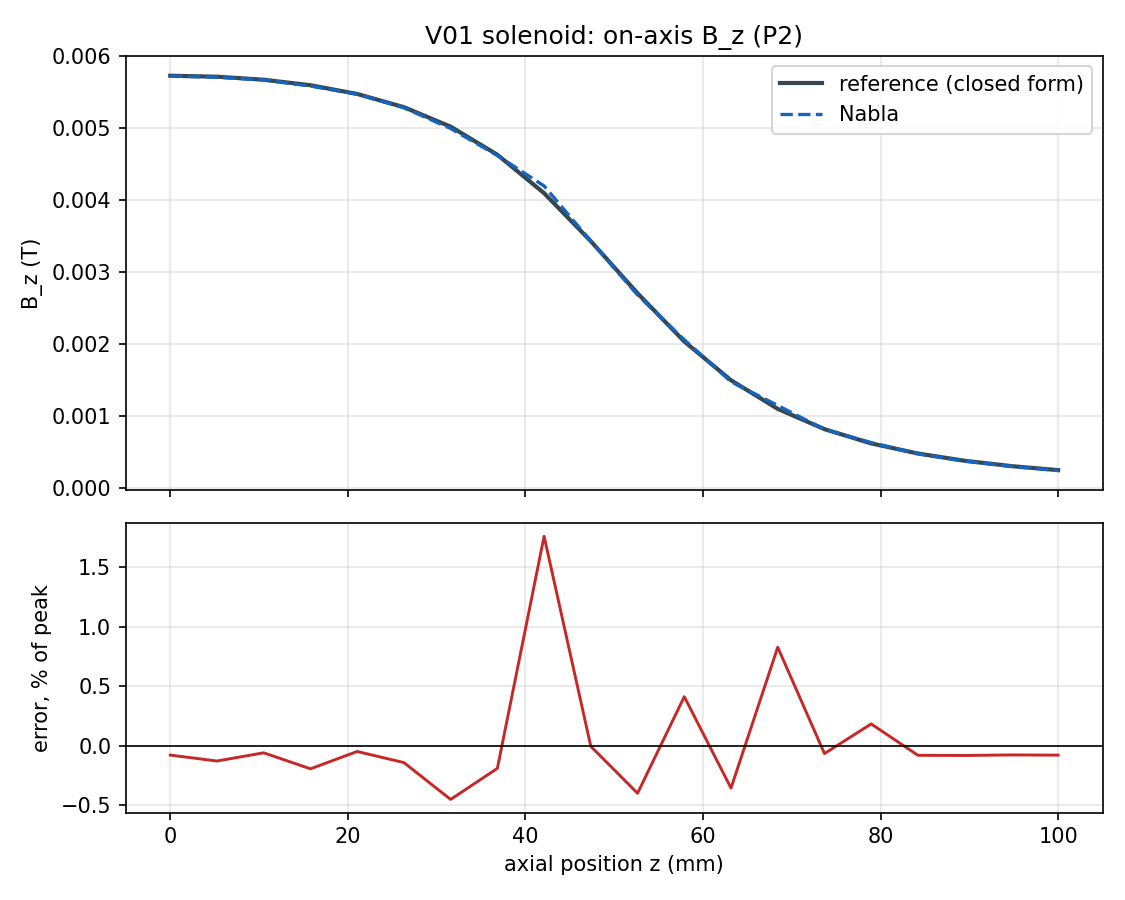
• Thick solenoid and ring, on axis. The exact field of a uniformly wound coil of rectangular section, B_z(z) = (mu0*J/2)*[f(b-z) + f(b+z)], f(u) = u*ln((r2 + sqrt(r2^2+u^2)) / (r1 + sqrt(r1^2+u^2))). This, not mu0*n*I, is the reference: a finite model must be compared against the finite answer. For this solenoid the infinite formula gives 6.2832 mT against the true 5.7288 mT - a 9.7 % difference that is physics, not error.
• Flux through a coaxial circle. Phi = 2*pi*rho*A_phi, with A_phi from Maxwell's elliptic-integral filament potential integrated over the winding cross-section by Gauss-Legendre quadrature.

Source statement as frozen: Closed form. Ampere's law for the round conductor; the exact on-axis field of a coil of rectangular section for the solenoid and the ring; Maxwell's elliptic-integral vector potential for the flux. All evaluated by harness/analytic.py - see chapter section 2. Tolerances are transcribed from the validation plan, case V01.

3. Nabla model

Built entirely through nabla_api by build.py in this directory - no GUI step, no manual edit. Meshes for this run:

Sub-model	Element order	Nodes	Elements
coax	P1	6381	12400
solenoid_p2	P2	20450	10123
solenoid_p1	P1	5164	10123
loop	P2	20217	10024

Every sub-model stays under the free tier's 25 000-node cap, so this case can be reproduced without a licence. The models themselves are published beside this chapter under artifacts/models/.

4. Results

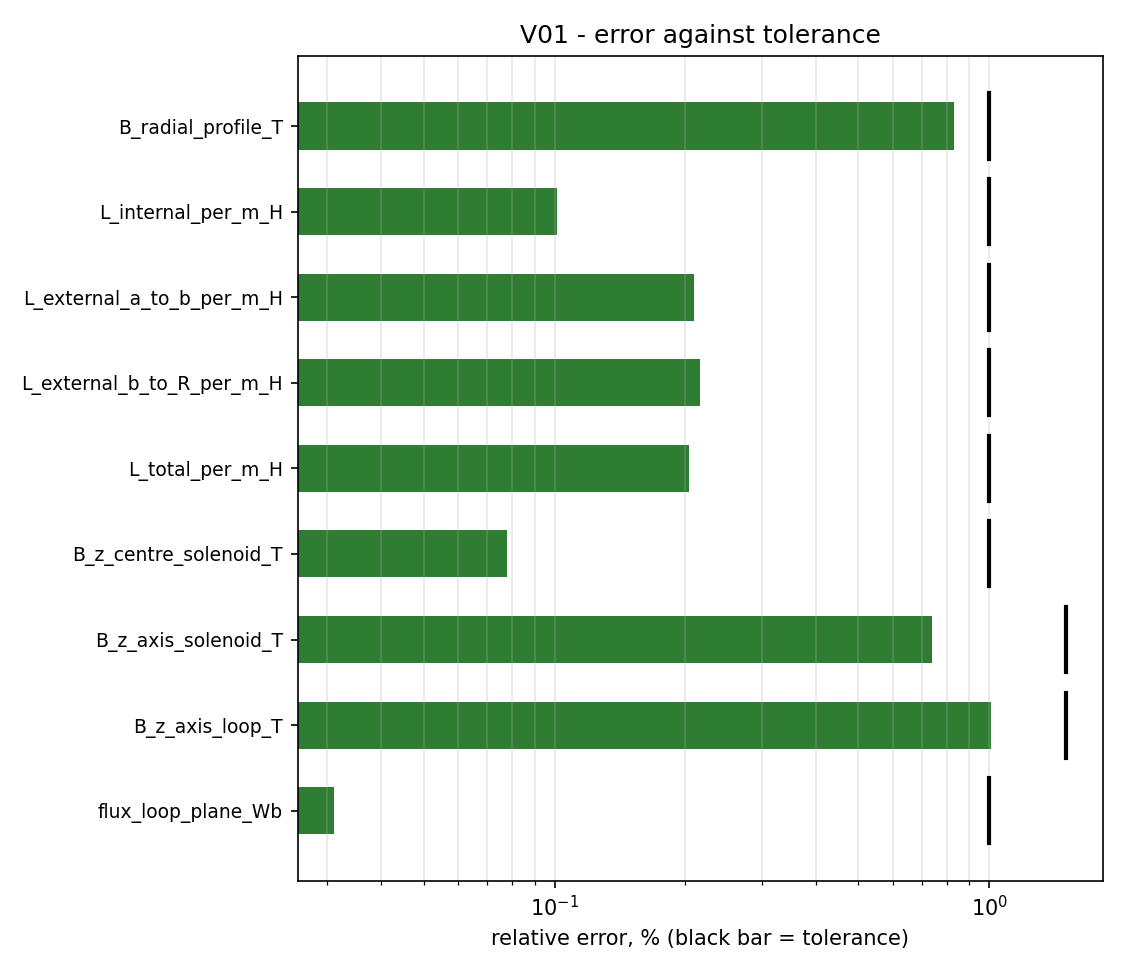
Quantity	Metric	Nabla	Reference	Error	Tolerance	Verdict
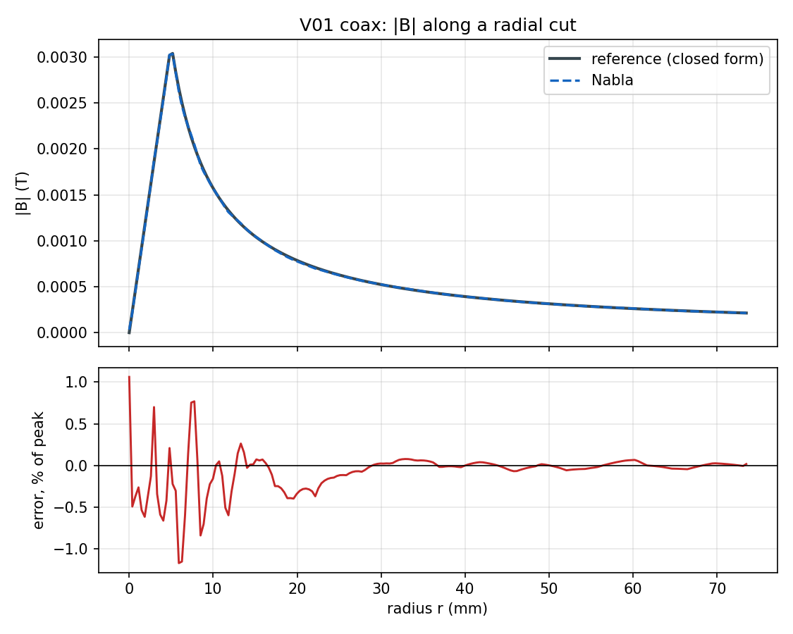
B_radial_profile_T	profile	min=3.223e-05, max=0.003031, rms=0.0009157 T	min=0, max=0.003038, rms=0.0009191 T	L2 +0.830 %, max +1.171 %	L2 1.000 %, max 2.000 %	PASS
L_internal_per_m_H	rel	4.99494e-08 H/m	5e-08 H/m	-0.101 %	1.000 %	PASS
L_external_a_to_b_per_m_H	rel	2.19262e-07 H/m	2.19722e-07 H/m	-0.209 %	1.000 %	PASS
L_external_b_to_R_per_m_H	rel	3.21193e-07 H/m	3.21888e-07 H/m	-0.216 %	1.000 %	PASS
L_total_per_m_H	rel	5.90405e-07 H/m	5.9161e-07 H/m	-0.204 %	1.000 %	PASS
B_z_centre_solenoid_T	rel	0.00572433 T	0.00572879 T	-0.078 %	1.000 %	PASS
B_z_axis_solenoid_T	profile	min=0.0002378, max=0.005724, rms=0.003732 T	min=0.0002423, max=0.005729, rms=0.003732 T	L2 +0.739 %, max +1.762 %	L2 1.500 %, max 3.000 %	PASS
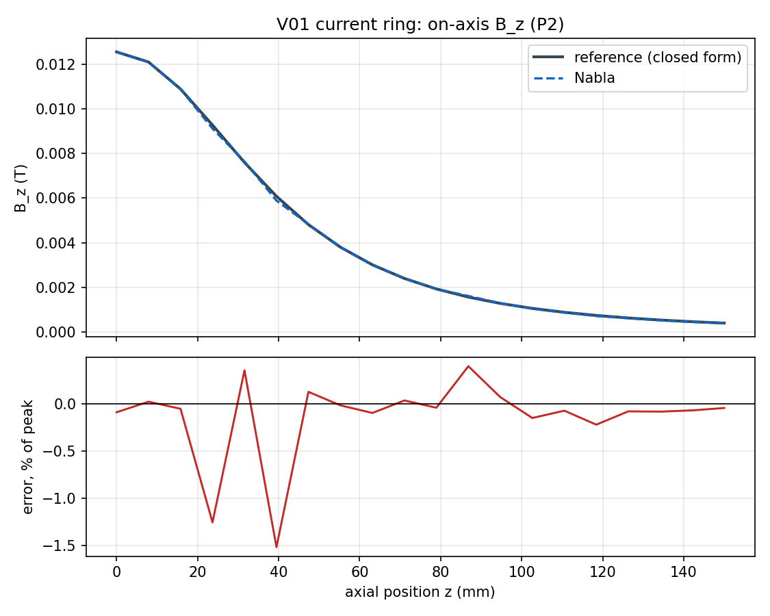
B_z_axis_loop_T	profile	min=0.0003928, max=0.01253, rms=0.005751 T	min=0.0003985, max=0.01254, rms=0.005772 T	L2 +1.010 %, max +1.520 %	L2 1.500 %, max 3.000 %	PASS
flux_loop_plane_Wb	rel	2.73619e-05 Wb	2.73704e-05 Wb	-0.031 %	1.000 %	PASS
B_z_centre_solenoid_P1_T	rel	0.00803628 T	0.00572879 T	+40.279 %	-	REPORT
B_z_offaxis_solenoid_P1_T	rel	0.00577219 T	0.00572879 T	+0.758 %	-	REPORT

5. Discussion

The energy-derived inductances are the strongest result here: L_internal lands at -0.101 % of mu0/(8*pi), which exercises the region energy integral, the axial-length convention and the unit handling in one number. The radial |B| profile is worst at r = a, where the field's radial derivative is discontinuous and a P1 solution can only average across the interface; the L2 error over the whole cut is +0.830 % against a 1 % tolerance.

The one result worth reading twice is the pair of rows published without a verdict. Probing B_z at the centre of the solenoid, exactly on the symmetry axis, gives +40.279 % at P1 and -0.078 % at P2. Move the same P1 probe 2 mm off the axis and the error collapses to +0.758 %. The solution itself is fine at P1 - the flux, which reads the primary unknown, is accurate to well under a percent - but the axisymmetric formulation stores u = r*A_phi and recovering B_z = (1/r) du/dr at r = 0 is a 0/0 that the linear element cannot resolve. P2 carries the axis-node Hessian recovery that can. Refining the P1 mesh does not fix it: across a 12x refinement sweep the on-axis error moved +40 %, -0.3 %, +31 % - noise, not convergence.

On-axis recovery stays somewhat mesh-sensitive even at P2: three meshes of the ring model at 20 k, 22 k and 29 k nodes gave L2 errors of 1.01 %, 1.14 % and 0.66 %. The coarsest of the three is the one shipped, which is a deliberate choice to keep the case reproducible on the free tier rather than a tuned result - the model parameters are in build.py for anyone who wants to check.

6. Limitations

• Do not probe B on the symmetry axis of an axisymmetric model at P1. Use P2, or probe a short distance off the axis. Integral quantities (flux, energy, force) are unaffected at either order.
• Linear materials only: mu_r = 1 everywhere. Nonlinear BH is V02 and V21.
• Static, no eddy currents, no motion, no circuit. Those are V11, V12 and V04.
• The coax sub-model carries no return conductor, so it validates the field of a single round conductor rather than the coupled two-conductor line.
• The reference for the ring is exact for a uniform current density over a rectangular section, which is what the model imposes - it is not a filamentary loop, and the textbook filament formula is quoted in the chapter only for context.

7. Reproduce

cd validation
python -m harness.run_case V01

Requires a built triangle.exe (Nabla does not distribute it) and a solver binary. Artifacts, including the four models, land in cases/V01_coax_solenoid/artifacts/.

8. Changelog of the frozen reference

No entry: the reference values and tolerances are as first frozen.