V02 — C-core electromagnet with an airgap

← Back to the validation dossier

Tier A+X (analytic + cross-code) - priority P0 Reference frozen on 2026-08-08. Nabla 0.1.0, solver licence mode enforcing, run in 116.2 s.

1. Problem

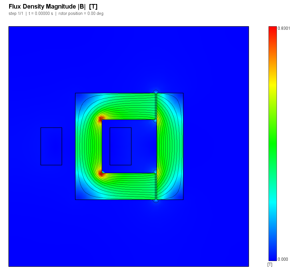
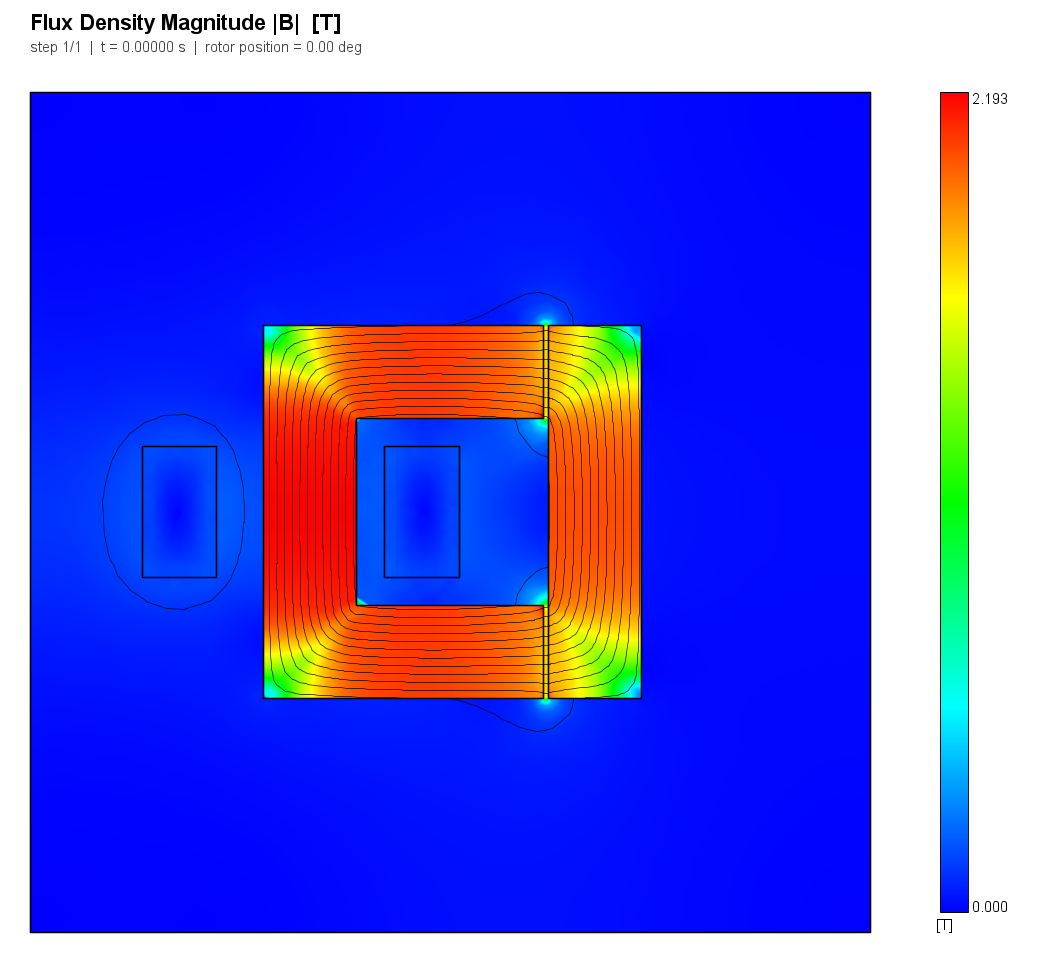
A wound C-core facing a flat armature across an airgap: the simplest device in which iron carries most of the flux, a gap carries most of the reluctance, and the answer changes qualitatively once the steel saturates. Twelve solves.

Sub-model	Iron	Gap	Excitation	What it is for
linear	mu_r = 1000	1 mm	2000 A-turns	the branch the reluctance sketch is written for
ni0 .. ni7	M-36 steel	1 mm	500 .. 12000 A-turns	unsaturated through the knee to hard saturated
gap0p5, gap2, gap4	M-36 steel	0.5, 2, 4 mm	2000 A-turns	the airgap sweep (1 mm is ni3)

Core 60 x 80 mm with a 40 x 40 mm window, 20 mm legs; armature 20 mm thick; 400-turn coil with its go side in the window and its return side outside the core; 50 mm deep; A = 0 on a box at -50..130 mm in both directions. Every one of those numbers lives once, in geometry.json, which the FEMM reference generator reads as well.

The excitation stops at 12000 A-turns on purpose. Beyond that the working point leaves the M-36 table (which ends at 2.3 T) and the two codes would be comparing their own extrapolation rules rather than the material.

2. Reference

Three references of three different strengths, and the chapter is explicit about which number rests on which. The case's reference notes set out the full statement.

Exact - Ampere's law. The closed integral of H.dl around a rectangle lying entirely in the window air, enclosing the go-coil and nothing else, is the enclosed N*I exactly - whatever the iron is doing. That makes it the one analytic check that survives saturation, and it tests the nonlinear H(B) inversion and the field solution together. Both codes assemble H.dl from Hx and Hy at the same 160 midpoint stations and integrate it themselves; neither code's own tangential-component sign convention is used.

Cross-code - FEMM 4.2. The identical model, built by pyfemm from the same geometry.json and the same BH table, with every compared quantity defined identically on both sides. The FEMM run is a reference generation step whose output is frozen into expected.json, so the nightly gate needs no FEMM installation and the third-party answer cannot move under the case between runs.

That the two codes really did get the same curve is not asserted, it is measured: the case reads the BH table back out of the running Nabla model and compares it against the snapshot FEMM was given, point by point (bh_table_max_rel_diff_H, 5.45328e-08 against a 1e-5 tolerance - which is the 32-bit storage of the table, not a difference in it).

Reported, never judged - the lumped reluctance model. Series reluctances with a Carter-style fringing correction, and F = 2 * B^2 * A / (2 mu0) for the pull. It is the model an engineer sketches before opening a field solver. Nabla is the better answer there, so those rows carry no tolerance: a pass/fail against an approximation would be a claim about the approximation.

Source statement as frozen: Two references of different strength, plus one published without a verdict. (1) EXACT: Ampere's law on a rectangle lying entirely in the window air and enclosing only the go-coil - the closed integral of H.dl is the enclosed N*I whatever the iron is doing, which makes it the one analytic check that survives saturation. (2) CROSS-CODE: FEMM 4.2, driven by pyfemm, on a model built from the same geometry.json and the same BH table, with every compared quantity defined identically in both codes (reference/femm_ccore.py, output frozen in reference/femm_reference.json). (3) REPORTED, NOT JUDGED: the lumped reluctance model with a Carter-style fringing correction, which is an approximation - Nabla is the better answer there, so a pass/fail against it would be a claim about the approximation. Tolerances are transcribed from the validation plan, case V02.

3. Nabla model

Built entirely through nabla_api by build.py - no GUI step, no manual edit. The nonlinear branch uses the shipped library material M-36_steel rather than a curve this case typed in, so what Nabla saturates on is a shipped artifact. Saturation is enabled for every configuration including the linear branch, so the nonlinear path has to reproduce a constant-mu_r material rather than being bypassed.

The airgap refinement rule was fixed before any run: the gap-facing boundaries of the core and the armature are subdivided to min(gap/3, 1 mm), so even the 0.5 mm gap carries three element layers. Meshes for this run:

Sub-model	Element order	Nodes	Elements
linear	P1	5196	10260
ni0	P1	5196	10260
ni1	P1	5196	10260
ni2	P1	5196	10260
ni3	P1	5196	10260
ni4	P1	5196	10260
ni5	P1	5196	10260
ni6	P1	5196	10260
ni7	P1	5196	10260
gap0p5	P1	6251	12372
gap2	P1	4658	9186
gap4	P1	4505	8879

Every sub-model stays well under the free tier's 25 000-node cap, so this case can be reproduced without a licence. The models themselves are published beside this chapter under artifacts/models/.

4. Results

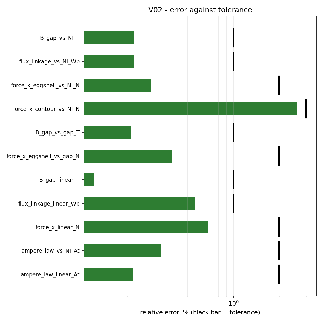
Quantity	Metric	Nabla	Reference	Error	Tolerance	Verdict
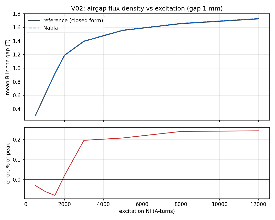
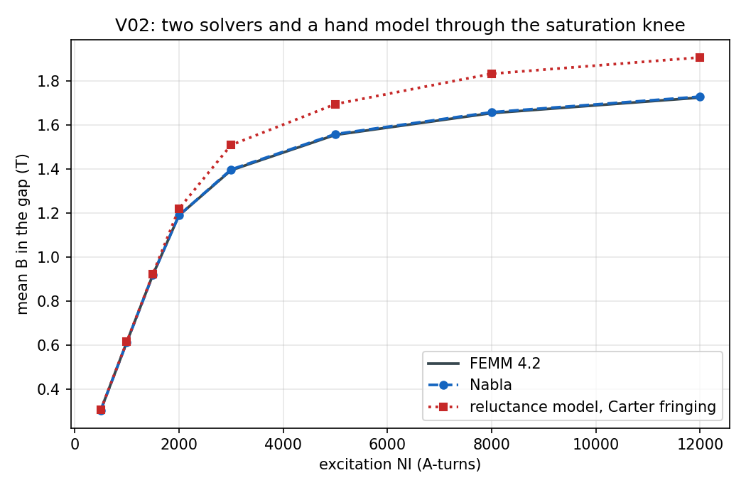
B_gap_vs_NI_T	profile	min=0.3055, max=1.729, rms=1.268 T	min=0.306, max=1.725, rms=1.266 T	L2 +0.222 %, max +0.245 %	L2 1.000 %, max 1.000 %	PASS
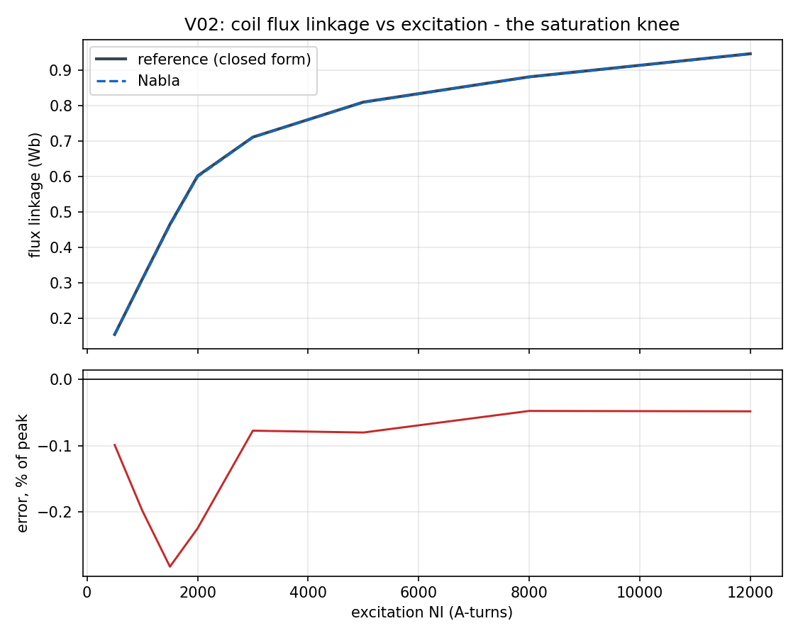
flux_linkage_vs_NI_Wb	profile	min=0.1539, max=0.9468, rms=0.6642 Wb	min=0.1549, max=0.9473, rms=0.6652 Wb	L2 +0.223 %, max +0.282 %	L2 1.000 %, max 1.000 %	PASS
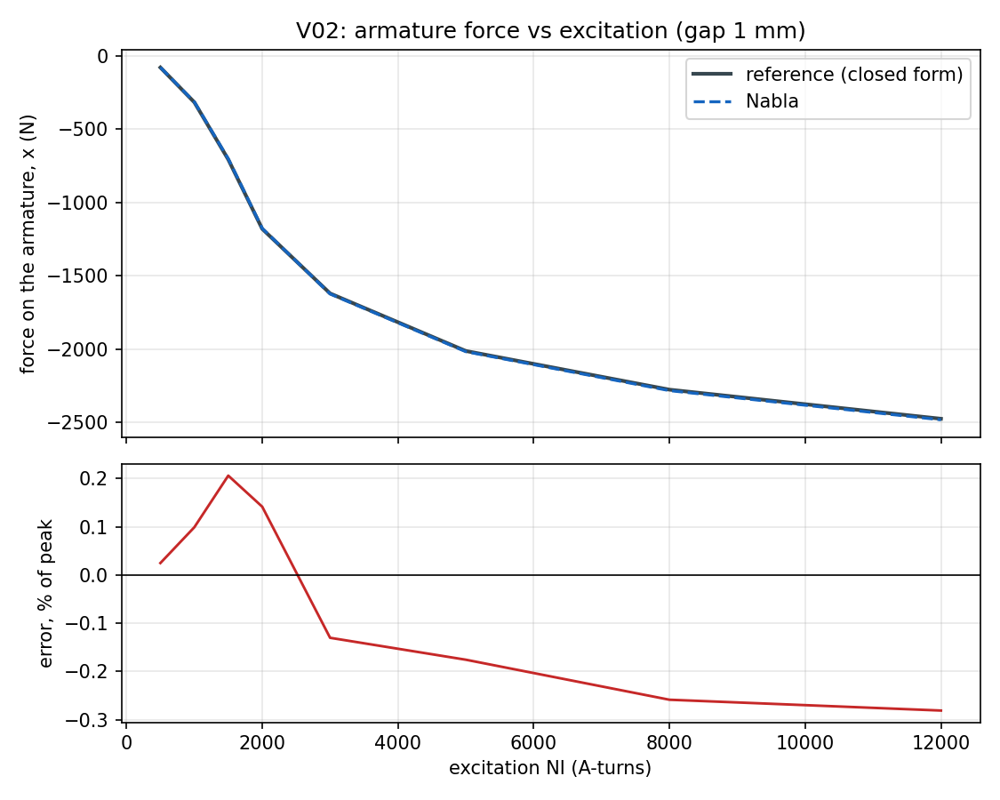
force_x_eggshell_vs_NI_N	profile	min=-2483, max=-77.51, rms=1584 N	min=-2476, max=-78.12, rms=1581 N	L2 +0.286 %, max +0.281 %	L2 2.000 %, max 2.000 %	PASS
force_x_contour_vs_NI_N	profile	min=-2567, max=-80.19, rms=1638 N	min=-2499, max=-79.21, rms=1596 N	L2 +2.622 %, max +2.709 %	L2 3.000 %, max 3.000 %	PASS
B_gap_vs_gap_T	profile	min=0.3077, max=1.515, rms=1.023 T	min=0.3086, max=1.511, rms=1.022 T	L2 +0.213 %, max +0.269 %	L2 1.000 %, max 1.000 %	PASS
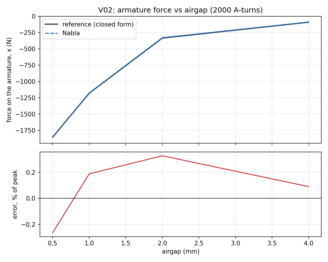
force_x_eggshell_vs_gap_N	profile	min=-1859, max=-87.24, rms=1113 N	min=-1854, max=-88.93, rms=1112 N	L2 +0.393 %, max +0.329 %	L2 2.000 %, max 2.000 %	PASS
B_gap_linear_T	rel	1.11356 T	1.11492 T	-0.122 %	1.000 %	PASS
flux_linkage_linear_Wb	rel	0.564033 Wb	0.567187 Wb	-0.556 %	1.000 %	PASS
force_x_linear_N	rel	-1030.02 N	-1037.12 N	+0.685 %	2.000 %	PASS
ampere_law_vs_NI_At	profile	min=499, max=1.196e+04, rms=5566 A-turns	min=500, max=1.2e+04, rms=5585 A-turns	L2 +0.333 %, max +0.334 %	L2 2.000 %, max 3.000 %	PASS
ampere_law_linear_At	rel	1995.65 A-turns	2000 A-turns	-0.217 %	2.000 %	PASS
bh_table_max_rel_diff_H	abs	5.45328e-08 -	0 -	5.453e-08	1e-05	PASS
B_gap_linear_over_reluctance	rel	1.00003 -	1 -	+0.003 %	-	REPORT
force_linear_over_reluctance	rel	0.974688 -	1 -	-2.531 %	-	REPORT
B_gap_over_reluctance_vs_NI	profile	min=0.9048, max=0.9971, rms=0.9532 -	min=1, max=1, rms=1 -	L2 +6.153 %, max +9.525 %	L2 -, max -	REPORT
force_method_agreement_vs_NI	profile	min=1.034, max=1.035, rms=1.035 -	min=1, max=1, rms=1 -	L2 +3.471 %, max +3.540 %	L2 -, max -	REPORT
newton_iterations_max	report	12 -	- -	-	-	REPORT
newton_final_residual_max	report	6.06494e-07 -	- -	-	-	REPORT

• newton_iterations_max: Nonlinear iterations of the worst of the twelve solves, counted from the solver's residual lines. Reported, never gated: an iteration count is a property of the Newton path, not of the answer
• newton_final_residual_max: Largest converged residual over the twelve solves, against the 1e-6 tolerance the models were configured with

5. Discussion

The field quantities are the strong result. Gap flux density agrees with FEMM to +0.222 % (L2) across the whole excitation sweep and +0.213 % across the airgap sweep, including the 0.5 mm gap. Coil flux linkage - the quantity that carries the saturation knee, and the one a designer actually uses - agrees to +0.223 %. Two independently written codes, two independent meshes, two different nonlinear solution strategies, one BH table.

Ampere's law is the check that matters most here, because it is the only one with no reference code behind it. The circulation reproduces the enclosed ampere-turns to +0.333 % (L2) over a sweep in which the iron goes from mu_r of several thousand to nearly nothing. A nonlinear solver that inverted B(H) inconsistently would fail this and could still pass a comparison against a code that made the same mistake.

The two force methods do not behave alike, and that is worth publishing. Nabla's eggshell region force matches FEMM's weighted stress tensor to +0.286 %; a mesh study on the 2000 A-turn point (3, 6 and 12 element layers across the gap - 5196, 6529 and 9325 nodes) had it converge monotonically at +0.30 %, +0.05 %, -0.03 %. The closed line contour on the same model did not converge at all: -3.20 %, -5.71 %, -3.87 % against that same weighted reference. A single closed-line integral of the Maxwell stress tensor across a 1 mm gap is a noisy object, and it is noisy in FEMM too - FEMM's own line contour sits 0.9 to 1.4 % away from FEMM's own weighted volume integral across the excitation sweep, and 3.2 % away at the 4 mm gap. That is one code disagreeing with itself by more than the two codes disagree on any field quantity in this chapter. Judged like for like (line against line) Nabla lands at +2.622 %; the two methods' own mutual disagreement is published as force_method_agreement_vs_NI, at +3.471 %. Use the eggshell.

Two modelling lessons came out of building this case, and both are in the published model rather than hidden by it:

• The stress contour was first drawn as a plain rectangle whose left edge ran up the mid-gap line for the whole 80 mm height. Over the 40 mm of open window that left it 0.5 mm from the armature in a region meshed at millimetres, so it sampled the first element layer: at 2000 A-turns it returned -1110.0 N against the like-for-like reference of -1193.2 N, an error of -7.0 %, where the published contour returns -1217.3 N, +2.0 %. The published contour runs mid-gap only across the two pole faces, where there is nowhere else to put it, and stands 5 mm off everywhere else. A stress contour must not be run through the first element layer of a body, and the stretch that faces no pole is where it is easiest to do that by accident.
• The frozen tolerance on the BH-table integrity check was originally absolute (1e-6 A/m). The table is stored in 32-bit floats and H reaches 215 kA/m, so that tolerance tested IEEE-754 rounding at the top of the curve and nothing at the bottom. It is now relative. Both edits are in the changelog below with their reasons, which is the mechanism this document is built on.

What the reluctance sketch is worth. On the linear branch it lands within +0.003 % of Nabla on gap flux density and -2.531 % on force - close enough that a first-pass sizing calculation is not wrong. Across the nonlinear sweep it drifts by +9.525 % at worst. That drift is the whole argument for solving the field: the sketch has no leakage, one guessed mean path length, and a fringing correction that is a fudge, and each of those matters more as the iron saturates.

6. Limitations

• Static, planar, no eddy currents, no motion, no circuit. Those are V04, V11 and V12.
• 1st-order elements only. V09 is the element-order study.
• The cross-code leg is a comparison, not an independent truth. FEMM is a well-respected code and this audience uses it, but two 2D FEM codes sharing a formulation can agree and both be wrong. That is exactly why Ampere's law is in this chapter: it is the row with nothing behind it but arithmetic.
• No hysteresis. The BH curve is single-valued, so the sweep is a magnetization curve and not a loop; remanence and minor loops are not modelled by either code here.
• The reluctance comparison is not a validation of anything. It is published to show the size of the error a lumped model makes.
• The armature force is the total force on the body, not a pressure distribution; V15 is the case that cross-checks the force methods against each other and against a closed form as its subject rather than as an aside.

7. Reproduce

cd validation
python -m harness.run_case V02

Requires a built triangle.exe (Nabla does not distribute it) and a solver binary. FEMM is not required: the cross-code numbers are frozen in expected.json. To regenerate them yourself, with FEMM 4.2 and pyfemm installed:

cd validation/cases/V02_ccore/reference
python femm_ccore.py

Artifacts, including the twelve models, land in cases/V02_ccore/artifacts/.

8. Changelog of the frozen reference

Date	Change	Reason
2026-08-08	bh_table_max_abs_diff_H_Am (absolute, tol_abs 1e-6 A/m) replaced by bh_table_max_rel_diff_H (relative, tol_abs 1e-5). No other reference or tolerance touched.	ModelData holds the BH table in 32-bit floats, and H on this curve runs from 19 to 215 229 A/m. An absolute tolerance of 1e-6 A/m therefore tested IEEE-754 round-trip at the top of the curve and nothing at all at the bottom - it would have failed on storage precision while a real 0.5 % divergence at low H slipped through. The relative form is scale-free: 1e-5 is two orders of magnitude tighter than any physically meaningful difference between two BH tables and an order of magnitude above float32 round-trip (~1.2e-7). The B column is still required to match to 1e-6 absolute, which float32 satisfies for B <= 2.3 T.
2026-08-08	force_x_contour_vs_NI_N re-pointed from FEMM's weighted VOLUME integral (block integral 18) to FEMM's LINE integral of the stress tensor over the same contour (mo_lineintegral(3)). The tolerance is unchanged at 3 %. No other quantity touched; the eggshell rows still compare against block integral 18.	The original pairing compared two different methods and called the difference solver error. Nabla's contour force came out +3.20 % against FEMM's weighted volume integral, and a mesh study (3 / 6 / 12 element layers across the gap, 5196 / 6529 / 9325 nodes) showed it does NOT converge with refinement - it moved -3.20 %, -5.71 %, -3.87 % - while the eggshell force on the same three meshes converged monotonically to +0.30 %, +0.05 %, -0.03 %. That is the well-known behaviour of a single closed-line stress integral, and FEMM shows it too: its own line contour differs from its own weighted volume integral by +1.15 % at this operating point. Judging Nabla's line integral against FEMM's volume integral therefore measured the gap between two methods, not the gap between two codes. The like-for-like reference was generated by extending reference/femm_ccore.py to walk the identical contour, and every previously frozen FEMM number was reproduced bit-for-bit by that re-run, which is recorded here because it is the thing that makes this edit auditable. The method-to-method difference has not been hidden: it is published in force_method_agreement_vs_NI and in the chapter's Discussion.