V17 — Circular loop self and mutual inductance, axisymmetric

← Back to the validation dossier

Tier A (analytic) - priority P1 Reference frozen on 2026-08-15. Nabla 0.1.0, solver licence mode enforcing, run in 52.1 s.

1. Problem

One circular loop, asked for its own inductance and for its coupling to eight others, in the axisymmetric formulation.

A single turn of 50 mm mean radius and 2 mm conductor radius carries 100 A. Eight identical turns sit coaxially above it at 10, 20, 30, 40, 50, 60, 80 and 100 mm - 0.2 to 2.0 loop radii - and carry nothing. The whole assembly is solved three times, in three different boxes.

Source	torus, R = 50 mm, conductor radius a = 2 mm, a/R = 0.04
Excitation	100 A over the round section, J = 7.9577 MA/m², linear, static
Receivers	eight identical tori at d = 10 ... 100 mm, air, no current
Formulation	Axisymmetric 2D, P2 (6-node quadratic elements)
dirichlet_20R	hemispherical domain, R_dom = 1000 mm = 20 R, A = 0
farfield_5R	R_dom = 250 mm = 5 R, far-field (balloon) BC, type 11, n = 1
dirichlet_5R	R_dom = 250 mm, A = 0 - the control

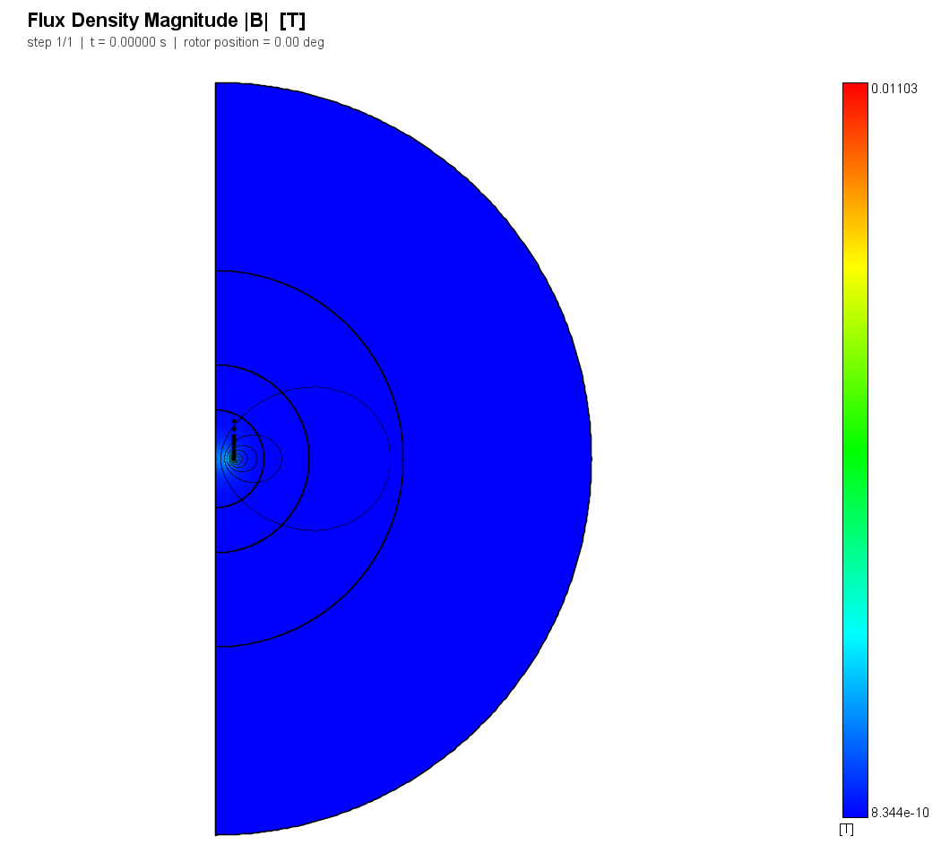
Why eight receivers and one solve. The receivers are air with mu_r = 1 and no current: they are magnetically invisible. In a linear magnetostatic problem they therefore cost nothing but the mesh they occupy, and one solve yields all eight mutual inductances instead of eight solves yielding one each. What makes them measurable rather than decorative is that an axisymmetric region flux is already the right integral - Results.calcFlux returns 2*pi times the area average of the flux function u = r*A_phi, which is exactly the flux linkage of one turn wound uniformly across that section. So

M_k = Flux(Recv_k) / I

with no geometry factor of the case's own invention in between.

Why axisymmetric at all. This is the formulation with the awkward integrand. The unknown is not the potential but r*A_phi; the stiffness kernel carries a 1/r, the field recovery divides by r again, and the axis is a coordinate singularity rather than a boundary. V01 exercises it on a probe value. This case exercises it on two integrals - one over a cross-section (flux) and one over the entire domain (energy) - and on the far-field boundary condition, whose axisymmetric variant carries its own 1/r weighting (the far-field boundary specification section 1.2) and had never been measured outside the file that implements it.

2. Reference

Derived in full in the case's reference notes. Three formulas and one deliberate refusal.

Mutual. Maxwell's exact result for two coaxial filaments,

M = mu0 sqrt(a b) [ (2/k - k) K(k) - (2/k) E(k) ],   k^2 = 4ab/((a+b)^2 + d^2)

evaluated with scipy.special.ellipk/ellipe. But a meshed loop is a torus and not a filament, and the case declines to compare one with the other: the reference is that formula averaged over both conductor cross-sections by product Gauss-Legendre quadrature, M = (1/(A_a A_b)) INT INT M_fil dA_a dA_b, which is the pairing the model actually contains.

Self. The classical thin-wire series for a uniform current density,

L = mu0 R ( ln(8R/a) - 2 + Y ),   Y = mu_r/4 = 1/4

= 222.947 nH. This one is an approximation, and the chapter says so twice rather than once, because the 2 % tolerance the validation plan gives it is a statement about the formula and not about the solver.

Source statement as frozen: Closed form throughout, evaluated in harness/analytic.py (section: circular filament, and section: circular loop of ROUND cross-section). MUTUAL: Maxwell's exact mutual inductance of two coaxial circular filaments, M = mu0sqrt(ab)((2/k - k)K(k) - (2/k)E(k)) with k^2 = 4ab/((a+b)^2 + d^2), evaluated with scipy.special.ellipk/ellipe. A meshed loop is a torus and not a filament, and what an axisymmetric region flux returns is the area average of 2piu over the receiver's cross-section, so the reference is that filament formula averaged over BOTH conductor sections by product Gauss-Legendre quadrature (mutual_inductance_loops): M = (1/(A_a A_b)) INT INT M_filament dA_a dA_b. At a/R = 0.04 that finite-section average sits 0.03 to 0.06 % above the bare filament value, and the filament value is published beside it without a verdict so a reader can see the size of the approximation this case declined to make. SELF: the classical thin-wire series for a circular loop of round cross-section carrying a uniform current, L = mu0R(ln(8R/a) - 2 + Y) with the internal (Neumann) flux term Y = mu_r/4 = 1/4. It is an approximation, dropping terms of order (a/R)^2 ln(R/a); Grover's next term, L = mu0R*((1 + a^2/(8R^2))ln(8R/a) + a^2/(24R^2) - 2 + Y), is published as a second reference without a verdict, and the 0.032 % between the two IS the formula's own uncertainty at this aspect ratio. Model: R = 50 mm, a = 2 mm, 100 A, one source at z = 0 and eight receivers at 10 ... 100 mm, axisymmetric, P2. Tolerances are transcribed from the validation plan, case V17: M <= 1 %, L <= 2 %.

3. Model and mesh

Sub-model	Element order	Nodes	Elements
dirichlet_20R	P2	81664	40633
farfield_5R	P2	61030	30349
dirichlet_5R	P2	61030	30349

Two mesh decisions are worth stating because both were mistakes first.

The conductor is a 96-gon, not a 32-gon. The source carries a fixed current density, so the current it delivers is J times the area the mesher gave it. A regular n-gon inscribed in a circle is short by 1 - (n/2pi) sin(2pi/n), which is 0.64 % at n = 32 - and the case's first run duly reported a flat -0.65 % on every one of the eight mutual inductances. That is a geometry error, not a discretization error, so it is removed by subdivision rather than reported as solver error, exactly as V01 removes the same error from its coax. At n = 96 it is 0.07 %, an eighth of the tightest tolerance here.

Every torus wears a 4 mm collar of fine air, and 4 mm is a maximum rather than a taste. The loops are 10 mm apart; the collars were 6 mm in the first draft, so adjacent collars intersected. An unsplit crossing in the PSLG is not an error Triangle reports - it meshed, it solved, and it silently leaked the source region's attribute into its own collar, giving the "100 A" conductor an area of 60.1 mm² instead of 12.5 and a current of 478 A. Section 6 is about how that was caught.

The axis and the grading rings follow the PSLG rule that the far-field boundary specification's axisymmetric phase records: the rings are open arcs terminating on shared axis vertices, and r = 0 is one chain split at every ring radius. Drawn as closed half-discs instead, each ring lays a second segment on top of the axis and Triangle hangs rather than complaining.

4. Results

Quantity	Metric	Nabla	Reference	Error	Tolerance	Verdict
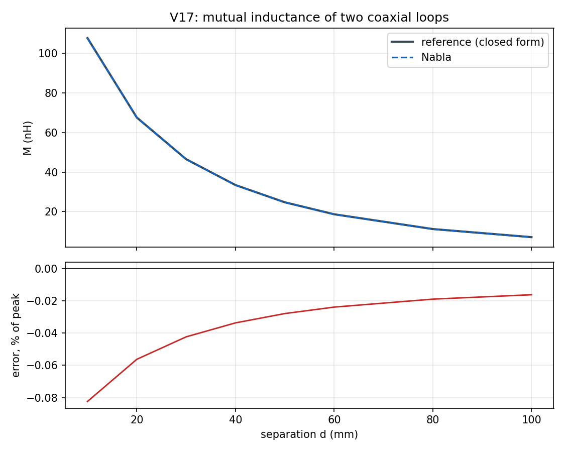
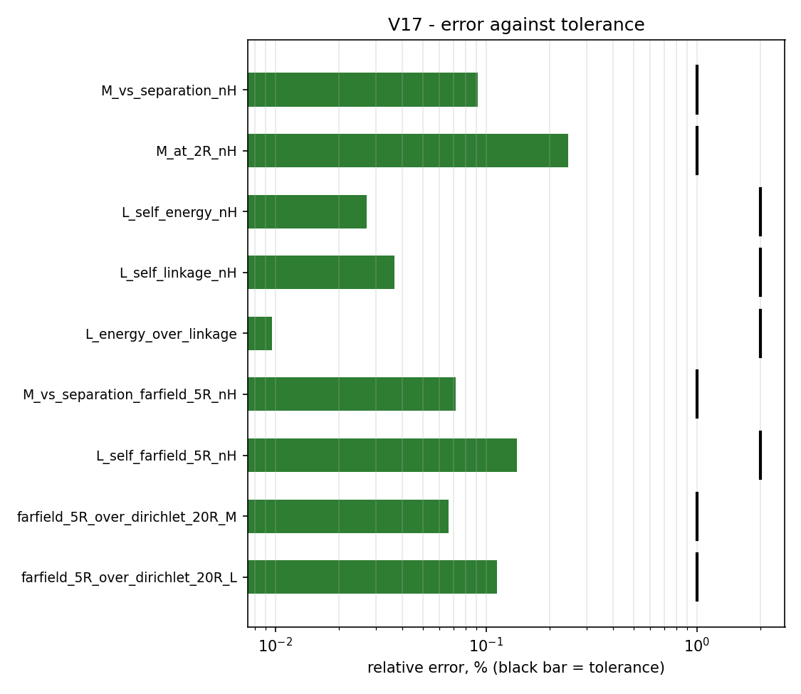
M_vs_separation_nH	profile	min=7.08, max=107.6, rms=50.68 nH	min=7.097, max=107.7, rms=50.73 nH	L2 +0.091 %, max +0.082 %	L2 1.000 %, max 1.000 %	PASS
M_at_2R_nH	rel	7.08006 nH	7.09747 nH	-0.245 %	1.000 %	PASS
M_vs_separation_filament_nH	profile	min=7.08, max=107.6, rms=50.68 nH	min=7.093, max=107.7, rms=50.71 nH	L2 +0.056 %, max +0.051 %	L2 -, max -	REPORT
L_self_energy_nH	rel	222.887 nH	222.947 nH	-0.027 %	2.000 %	PASS
L_self_linkage_nH	rel	222.865 nH	222.947 nH	-0.037 %	2.000 %	PASS
L_energy_over_linkage	rel	1.0001 -	1 -	+0.010 %	2.000 %	PASS
L_self_grover_nH	rel	222.887 nH	223.018 nH	-0.059 %	-	REPORT
M_vs_separation_farfield_5R_nH	profile	min=7.09, max=107.7, rms=50.69 nH	min=7.097, max=107.7, rms=50.73 nH	L2 +0.072 %, max +0.071 %	L2 1.000 %, max 1.000 %	PASS
L_self_farfield_5R_nH	rel	222.635 nH	222.947 nH	-0.140 %	2.000 %	PASS
farfield_5R_over_dirichlet_20R_M	profile	min=1, max=1.001, rms=1.001 -	min=1, max=1, rms=1 -	L2 +0.067 %, max +0.134 %	L2 1.000 %, max 1.000 %	PASS
farfield_5R_over_dirichlet_20R_L	rel	0.998872 -	1 -	-0.113 %	1.000 %	PASS
M_vs_separation_dirichlet_5R_nH	profile	min=6.31, max=106.9, rms=50.08 nH	min=7.097, max=107.7, rms=50.73 nH	L2 +1.609 %, max +0.804 %	L2 -, max -	REPORT
L_self_dirichlet_5R_nH	rel	222.109 nH	222.947 nH	-0.376 %	-	REPORT
dirichlet_5R_over_dirichlet_20R_M	profile	min=0.8912, max=0.9928, rms=0.9618 -	min=1, max=1, rms=1 -	L2 +5.043 %, max +10.880 %	L2 -, max -	REPORT
dirichlet_5R_over_dirichlet_20R_L	rel	0.996509 -	1 -	-0.349 %	-	REPORT

5. Reading

The mutual inductance is right to a tenth of a percent. Over the whole sweep the L2 deviation is +0.091 % against a 1 % tolerance, and the per-point error grows monotonically from -0.08 % at d = 0.2R to -0.245 % at d = 2R, where the coupling has fallen by a factor of 15 and the boundary is nearest. The monotone growth is the signature of truncation rather than of the mesh: the weakest coupling is the one a finite box distorts most, and section 7 measures exactly that.

The separate M_at_2R_nH row exists because the profile metric normalises its pointwise error by the peak of the reference. A 1 % error on the 7 nH tail would disappear inside a tolerance set by the 108 nH head, so the far end of the sweep is judged on its own value as well.

The self-inductance lands inside the reference formula's own uncertainty. Nabla reads 222.887 nH from field energy and 222.865 nH from flux linkage, against 222.947 nH from mu0 R (ln(8R/a) - 2 + 1/4): errors of -0.027 % and -0.037 % against a 2 % tolerance. Grover's (a/R)^2-corrected series gives 223.018 nH, so the two analytic values differ by 0.032 % - and Nabla sits between them. At this aspect ratio the honest statement is not "Nabla agrees with the formula to 0.03 %" but "Nabla and the formula agree to within the formula's own truncation, and neither one is demonstrably the better answer". The crossover the plan asks for is therefore already behind us at a/R = 0.04: the thin-wire series loses its last digit around a/R ~ 0.1, where its dropped (a/R)^2 ln(R/a) term reaches half a percent, and beyond that the field solution is the better number.

The finite cross-section matters more than the discretization. Against the bare filament formula - the one the plan names, and the one this case declined to use - Nabla's eight numbers deviate by +0.056 % (L2). Against the cross-section-averaged reference, +0.091 %. The 0.03 to 0.06 % between the two is what treating a 2 mm conductor as a filament costs, and it is comparable with the solver error it would otherwise have been confused with. This is the same lesson V01 records for the thick solenoid, in the one place a reader is most likely to reach for a textbook formula without checking which geometry it describes.

6. The identity row, and what it caught

L_energy_over_linkage divides 2W/I^2 by lambda/I, and reads +0.010 % from unity. For a uniform current density in a bounded domain W = lambda I / 2 exactly, so this row is a discrete identity between two post-processors and not independent evidence for either - V15 records the planar version of it agreeing to 6e-12, and this chapter would be over-claiming if it counted the energy and the linkage as two results.

It is worth its place for a different reason. Both sides of the identity assume the same current, but they assume it with different powers: energy scales as I^2 and linkage as I. Their ratio is therefore I_true / I_assumed, and it is blind to almost everything else. On this case's first run it read 4.78 - which is 60.124 mm² / 12.573 mm², the ratio of the area Triangle gave the conductor to the area it was supposed to have, and the whole diagnosis of the overlapping-collar leak described in section 3. The mutual inductances were wrong by 4 to 10x at the same time, but they were wrong in a way that still looked like a field: monotone in separation, smooth, plausible. The identity row named the cause in one number.

Both findings — the polygon shortfall of section 3 and the collar leak — are written up with their evidence, their code pointers and a proposed Checklist advisory in case V17.

Anyone building an axisymmetric model with a current density rather than a coil should keep this ratio in view. It also catches an r weighting dropped on one side of the post-processing and not the other, which is the axisymmetric mistake most worth insuring against.

7. The far-field boundary, in axisymmetry, on integral quantities

Three boxes, one question: how much of the answer is the boundary?

	M at d = 0.2R	M at d = 2R	L
Dirichlet at 5 R	-0.72 %	-10.88 %	-0.35 %
Far-field at 5 R	+0.01 %	+0.13 %	-0.11 %

Both 5-radius models are the same geometry, the same mesh rule and the same solver settings; they differ in one boundary condition. Against the 20-radius Dirichlet reference model the balloon holds every mutual inductance to +0.134 % at worst and the self-inductance to -0.113 %, while the Dirichlet control in the same box loses 10.9 % of the weakest coupling. On that quantity the far-field condition is worth a factor of 80, and it buys back a domain four times smaller in radius - sixteen times smaller in area, and in the fully three-dimensional problem this rotates into, sixty-four times smaller in volume.

Two things this measurement adds to the far-field boundary specification's own Phase 4 table.

• It is on integral quantities - a flux linkage over a cross-section and an energy over the whole domain - rather than on a probe value, and it is measured by a script that knows nothing about the implementation.
• It shows the shape of the error. The Dirichlet box's deficit grows from 0.72 % to 10.88 % as the pair separates, because a distant, weakly coupled pair has more of its mutual flux out where the box has clamped A to zero. A truncation error is not a constant; it is largest exactly where the quantity is smallest, which is where a designer is least likely to notice it and most likely to be sizing a shield or a stray-coupling budget.

Note also the direction: the Dirichlet control reads low on every quantity, never high. A box that forces A = 0 too close in removes flux that should have closed outside it, and both the coupling and the stored energy fall. A truncation error that ever reads high is not truncation.

8. Limitations

• The receivers are magnetically invisible, by construction. Giving one a permeability, a conductivity or a closed turn would change the field, and one solve would stop being eight measurements. Nothing here validates a mutual inductance between coupled windings; V16 does that, with a circuit.
• No proximity effect. Every current in this case is an imposed uniform density and nothing redistributes. The frequency at which two loops 10 mm apart stop sharing current uniformly is V12's subject.
• L is measured, not derived from a coil. The source is a region with a Jz, not a Coil object with turns and a circuit; the turns count, the fill factor and the end-winding terms that a machine's inductance carries are not exercised here.
• This case cannot be run on the free tier. It uses P2 elements and the far-field BC, both licensed capabilities, and its meshes run to 82 k nodes against the free tier's 25 k cap. V01 covers the same axisymmetric formulation within those limits.
• The self-inductance tolerance is the formula's, not the solver's. 2 % is what the validation plan specifies for a thin-wire series; the measured disagreement is 0.03 %, and the two analytic orders disagree by 0.032 %. Do not read the 2 % as an estimate of Nabla's error on an inductance.

9. Reproduce

cd validation
python -m harness.run_case V17

The three models are published beside this chapter under models/, the eight separations and every series in series/, and the closed forms live in harness/analytic.py with their own tests in tests/test_harness.py.

Changelog

No entry: the reference values and tolerances are as first frozen.